Ever faced frustration with Excel formula errors? Understanding and fixing these errors doesn’t have to be a daunting task. This guide simplifies the process, showing common errors and how to correct them using Excel’s Formula Auditing tools. Sometimes, the solution is as straightforward as adding punctuation.
Like most software programs, there are multiple ways to find and fix errors. Some are specific, and others leave you confused, like the PivotTable field error. However, Excel seems to have added an extra layer of support for formula errors, including some tools to help you find a solution.
Quick Prevention Tips
Here are some tips for preventing errors. I find I make most of my formula errors when I go too fast. If I consciously slow down, my error rate decreases. But there are other prevention methods.
- Use the Functions Argument dialog – this is the built-in tool you can access when you use the Insert Function. While it may take a little more time, it will evaluate your formula, provide feedback, and link to function help. In the picture below, you can see the formula results in 2 places. Results are a good sign.

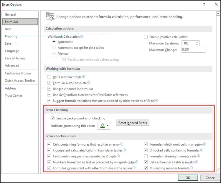
- Turn on Excel’s error checking. You can find these from the File | Options menu. This option checks and alerts you to some common mistakes.
- Remember the = sign – it’s easy to overlook this item if you type directly into the formula bar.
- Use quotes around text values – =CONCAT(“West”,A48).
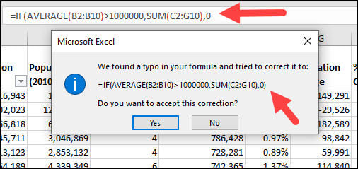
- Match your left and right parenthesis – =IF(AVERAGE(B2:B10)>1000000,SUM(C2:G10),0). The good news is if you typed this formula and omitted one of the parenthesis, Excel would catch this mistake.
Common Excel Formula Errors
Even if you take into account the prevention tips above, you’ll still see them. Excel has many formula errors, but let’s start with the most common ones.
#DIV/0!
This is the infamous divide by 0 or a blank cell error. Maybe it’s not infamous, but I’ve triggered it so often I did a separate tutorial on it. In the example below, I’m dividing by blank cells. I should’ve changed the formula in J2 to =B2/$K$2 before copying it down the column. That way, the “700000” entry in K2 would’ve been a constant divisor instead of adjusting as I moved down the column.

#N/A
Whenever I see N/A, I think of “not available” or “no answer.” In a sense Excel, is telling us the same thing. I tend to encounter this error when using a lookup function like VLOOKUP or XLOOKUP. In the example below, I’ve asked Excel to find the value for Pcode 24 from the Party Code spreadsheet. However, that specific code of “24” doesn’t exist on the Party Codes sheet.

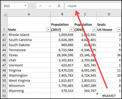
#NAME?
I tend to produce this error when I fail to complete the formula or have a typo. For example, I wanted to use the SUM function but forgot to include the cell references.
Another way to produce this error would be if I used =SUN(D2:D52). In this instance, Excel is saying it doesn’t recognize the SUN function.
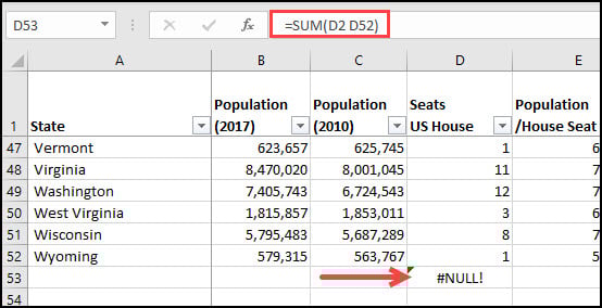
#NULL!
Excel formulas can be finicky about punctuation. In the example below, I omitted the colon between D2 and D52. In certain cases, such as summing multiple ranges, you can omit the colon.
#NUM!
This is one of those errors that occur in multiple situations. For example, Excel can only display numbers within a certain range. This is different than having a number wider than your column. However, we’re talking about huge numbers.
Another way I’ve produced this error is when I entered the wrong data type in a cell. This happens if I haven’t locked my column headers and think I’m in a different column. Too bad Excel data forms can’t handle formulas.
In the example below, I mistakenly entered -25 in a date field. Then when Excel tried to calculate the difference between the 2 dates, it failed. A similar problem happens when you try to do improbable math functions on a negative number.

#REF!
As the name hints, some reference is missing and the formula fails. I’ve been known to create this error when I’ve copied cell values from one place to another. In the example below, I copied the contents from cell D53, the simple SUM shown in the formula bar. However, when I paste D53 into L30, I lost my reference point.
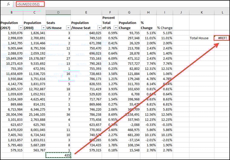
What’s annoying about this problem is when you hover over L30, you don’t know the formula.
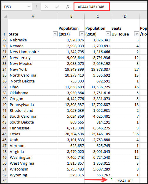
#VALUE!
This is Excel’s way of saying, “How do you expect me to get a value out of that formula?” Either I made a typo in the formula, or something is wrong with one or more cells. I’ve also had this error appear when converting or parsing a file and stray characters appear.
In the example below, I’m attempting to SUM three cells. However, cell D45 has a stray character that came in from a file import.
Formula Auditing
When I first learned Excel formulas, I concentrated on the Function Library group. It wasn’t till much later that I explored the Formula Auditing group. Clearly, a big mistake. Had I paid more attention, I would’ve found and fixed my mistakes much earlier. This toolbar group is invaluable if you inherit a spreadsheet and aren’t sure how it works.
The group sits on the Formula toolbar and includes a number of tools. I want to concentrate on several basic tasks.

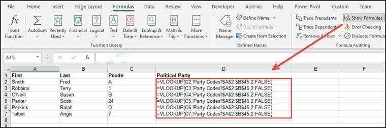
Show Formulas in Sheet
This tool is convenient when you revisit a spreadsheet you created or need to review one from someone else. Instead of hovering over cells and looking in the Formula bar, click Show Formulas. Any cell that contains a formula will show it instead of the results. You can see examples in Column D. Clicking the tool again reverts the cell contents back to the results.
Error Checking
It’s not uncommon for spreadsheets to have errors. It does help to scan your sheet for common errors using the Error Checking tool. The tool will scan the entire sheet and present one error at a time.
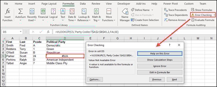
In the above example, cell D5 has an issue and produces a #NA error. If I want the Excel error help page, I can click Help on this Error. This versatile dialog also gets me to some of the other tools. For instance, I can jump to the Error Checking section on the Options panel. And, I can even pull up the formula and edit it.
Key Points & Takeaways
- Learn to recognize common mistakes, such as missing punctuation or incorrect syntax.
- Slowing down and using built-in tools like the Functions Argument dialog can decrease error rates.
- Explore the Formula Auditing group on the toolbar for tools like “Show Formulas in Sheet” and “Error Checking.”
- Don’t be intimidated by errors; experimenting with formulas and using built-in tools can lead to mastery.