In this XLOOKUP tutorial, you’ll learn how to streamline Excel data lookups and be more efficient. If you struggle to find matching data across worksheets or within large datasets, XLOOKUP can simplify your workflow. Start learning the basics of its syntax with this tutorial and practice file.
In fact, Microsoft recommends that you use it over VLOOKUP or HLOOKUP. The catch is that this lookup function is not available to all Excel users.
How to Get the Function
This function is only available with Microsoft 365 (Formally known as Office 365). So if you use one of the non-subscription versions of Microsoft Office or Excel, such as Excel 2019, you’re out of luck.
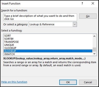
Go to your Formulas tab and click Insert Function to check your availability. The Insert Function dialog box will open with all your functions. XLOOKUP should show under the Lookup & Reference category between VLOOKUP and another new function called XMATCH.
Why is the XLOOKUP Function Better?
The question on most peoples’ minds is, what’s better? After all, who wants to learn something that doesn’t add value for Excel users. So here’s a shortlist I can see from playing around with various lookup scenarios:
- This function can work either vertically or horizontally. This is in contrast to the VLOOKUP function and HLOOKUP, which are mostly locked to their orientation.
- You’re not dependent on a sorted list.
- You don’t have to worry about the function breaking if you add or remove columns.
- It defaults to an exact match. If this is your preferred match type, then it’s one less argument you have to state.
- You’re not dependent on the first column.
- Your return array can be to the left of your lookup column.
There are more advantages to using wildcards, different search modes, and match modes like approximate matches. However, those are not covered in this introductory tutorial.
XLOOKUP Tutorial Example
I’ll use a simple Excel workbook with 2 sheets for this tutorial. You can download it from the Additional Resources section.
My goal is to populate Column C with the correct Periodic Table number that will be returned from Column H.
By default, XLOOKUP will perform an exact match mode on my stated lookup value, the element name. To do this, I’ll search off the common field “Name,” which appears in both ranges.
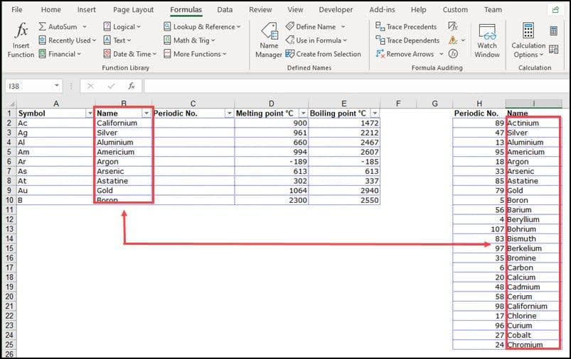
I’ve also added a second tab to the workbook called “Horizontal.” It contains the same information, but the data is laid out differently so you can see the function’s additional versatility. This worksheet also has the formula added.
You’ll also note that I’m adding the formula using Insert Function and the Function Arguments dialog box. I find this method easier when you’re learning a new function because it’s less likely to produce formula errors in Excel. But, there is nothing to prevent power users from using the formula bar and entering in a string like:
=XLOOKUP(B2,$I$2:$I$25,H2:$H$25)
Breaking Down the Function Syntax
The function has 5 arguments, but the last two are optional. These optional arguments are for “Match Mode” and “Search Mode.” Excel notes this by making the mandatory arguments in a bold typeface.
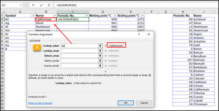
[A] The Lookup_value represents the cell Excel will use to find a corresponding value from the Lookup_array. For example, in this screenshot, we’ll look for “Californium” from cell B2. It is also noted in quotes to the right of the textbox.
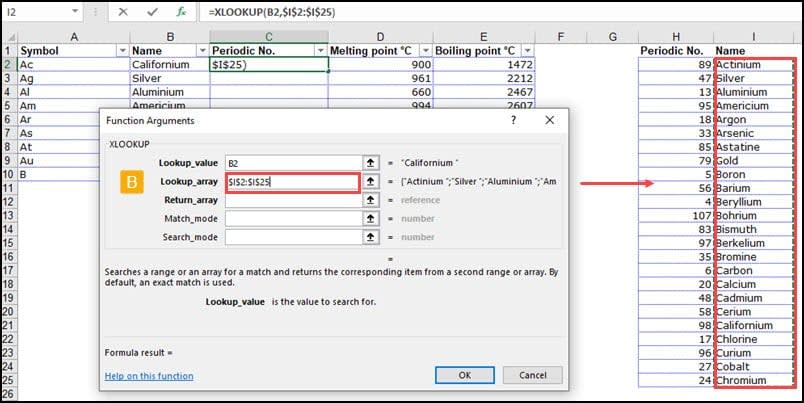
[B] The Lookup_array represents the cell range a matching Lookup_value can be found. In this example, we’re telling the application to lookup Californium from cell B2 and find the same value in column I. I added the $ signs to make an absolute range.
[C] The Return_array represents where our answers can be found. We’re telling Excel that once it finds the matching Californium from column I to go across and find the value from column H. In this example, I’m looking in a column to the left. I’ve highlighted the match in yellow.
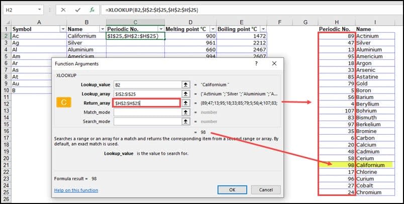
Once Excel matched Californium, it then looked up the Periodic No. The query returned 98, which shows at the bottom of the argument list, and the Formula result = line at the bottom.
How to Use XLOOKUP Step by Step
For this tutorial, I’ll be using Microsoft 365 and the xlookup-elements-examples.xlsx workbook. You can find it in the Additional Resources section. The workbook has 2 worksheets. One example is a common lookup, whereas the second one includes a horizontal lookup and the formula.
- Download the Excel file from the Additional Resources section.
- Select the Vertical worksheet.
- Click in cell C2. This is where we will put the lookup formula.
- Click the Formulas tab.
- Click Insert Function. The Insert Function dialog box appears.
- In the Search for a function: textbox, type xlookup.
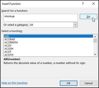
- Click Go.
- Click OK to accept XLOOKUP. A blank Function Arguments dialog appears.
- With your cursor in the Lookup_value field box, click cell B2. This is the field we want to match.
- Tab to advance to Lookup_array. This is the cell range that has matching values for column B.
- Select cells I2 through I25.
- Press F4 to make an absolute range.
- Tab to advance to Return_array. This is the range that contains our answers.
- Select cells H2 through H25.
- Press F4 to make an absolute range. You should see a result in the Formula result = line.
- Click OK. You should see 98 in cell C2.
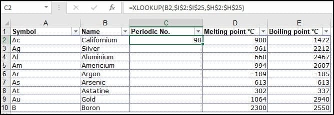
- With your cursor in cell C2, drag the fill handle to copy the XLOOKUP formula down the column.
In this XLOOKUP tutorial, you’ve gained a solid foundation in XLOOKUP syntax and discovered practical ways to simplify your Excel tasks. Still, don’t worry if you want to use VLOOKUP and HLOOKUP. Microsoft doesn’t have any plans to retire these functions. However, I think you’ll seldom use those functions now that you know how to use XLOOKUP in Excel. Why not download the practice file below and apply the concepts you’ve learned?
