Do you need to convert columns to rows in Excel? Transposing data is a common task for Excel users. I’ll show you how to quickly switch columns and rows using several efficient methods, including Paste Special and the TRANSPOSE function. You’ll learn techniques for switching your layout to improve your spreadsheet organization and make your data easier to analyze and visualize. (Includes video and practice file.)
Knowledge You’ll Gain:
By the end of this tutorial, you will be able to:
- Learn to transpose data using Excel’s Paste Special feature.
- Understand how to switch rows and columns with the TRANSPOSE function.
- Discover keyboard shortcuts for transposing data efficiently.
- Copy and paste transposed data to a new location in your sheet.
- Apply these techniques to switch rows and columns in any Excel version.
The Layout Problem in Excel
I was recently given a large Microsoft Excel spreadsheet that contained vendor evaluation information. The information was useful, but I couldn’t use tools like Auto Filter because of the way the data was organized. I would also have issues if I needed to import the source table into a database. A simple example is shown below.

Instead, I want to have the Company names displayed vertically in Column A and the Data Attributes displayed horizontally in Row 1. This would make it easier for me to do the analysis. For example, I can’t easily filter for California vendors with the original table.
About the Transpose Function
In simple terms, the transpose feature changes your columns’ orientation (vertical range) and rows (horizontal range). My original data rows would become columns, and my columns would become rows. So this fixes my layout problem above without me having to retype my original data. And the system would adjust for column labels.
The transpose function is pretty versatile. For example, you can use the feature in Excel formulas or with paste options. However, there are some differences based on which method you use.
Transposing with Paste Special
The steps outlined below were done using Microsoft Office 365, but recent Microsoft Excel versions will work.
- Open the spreadsheet you need to change. You may also download the example sheet at the end of this tutorial.
- Click the first cell in your cell range, such as A1.
- Shift-click the last cell of the range. Your data set should be highlighted.
- From the Home tab, select Copy or type Ctrl + c.

- Select the new cell where you would like to copy your transposed data.
- Right-click in that cell and select the Transpose icon from the Paste Options.

The data layout changes as you hover over the Paste options.
You should now see Excel switched the columns and rows. You can resize your columns to suit your needs.
These two data sets are independent. You can delete cells from the top set, and it will not impact the transposed set.

When using this method, your original formatting is maintained. For example, if I added a yellow background to my original cells B1:G1, the same background color would be applied. The same is true if I used red text on cell E:5.
Using Transpose in Formulas
As I mentioned, Excel has multiple ways for you to switch columns to rows or vice versa. This second way utilizes a formula and array. The result is the same, except your original data and the new transposed data are linked. As a result, you may lose some of your original formatting. For example, colored text and styles came across, but not cell fill colors.
- Open your Excel sheet.
- Click a blank cell where you want your converted data. I’m using A7.
- Type =transpose.
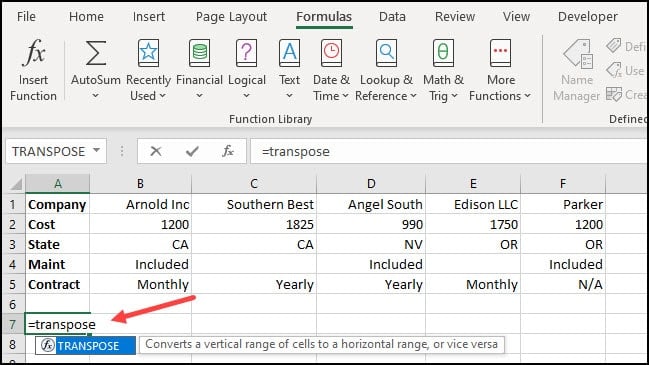
Notice how Excel provides a tooltip showing for Transpose – “Converts a vertical range of cells to a horizontal range and vice versa“.
- Finish the formula by adding a ( and highlighting the Excel cell range we wish to swap.
- Type ) to close the range.

- Press Enter.
If you’re not using Microsoft 365, you’ll probably need to press CTRL + SHIFT + Enter
Comparing Transpose Options
While these two methods produce similar results, there are differences. In the first paste method, whatever action I take on a cell is independent of the transposed version. I could delete the original values, and nothing would happen to the columns I swapped.
TextExpander: Worth It? Find Out.
Is TextExpander the right tool to boost your productivity? Get an independent assessment, weigh the pros and cons, and make an informed decision. Find out why I’m a fan.
Read the ReviewIn contrast, the Transpose formula version is tethered to the original data. So, for example, if I change the value in B2 from 1200 to 1500, the new value will automatically update in B8. However, the reverse isn’t true. If I change any transposed cells, the original set will not change. Instead, I will get a #SPILL error, and my transposed data will disappear.

Now that we’ve shown you how to transpose data in Excel, try playing around with the practice worksheet below. You’ll be swapping your rows and columns in Excel in no time. And while you likely work with multiple rows, you can convert one Excel column to a row.
Transpose and Blank Cells
Another difference with the Transpose formula is that it will convert blank cells to “0”s.
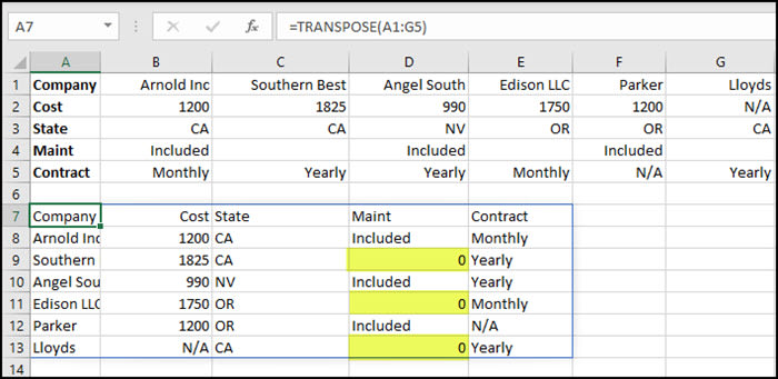
The fix for this quirk is to use an Excel IF statement in the formula that keeps the blank cells as blanks. You can hover over the box below to copy the transpose formula.
=TRANSPOSE(IF(A1:G5="","",A1:G5))
Alternatively, you could search and replace the zeros.
Show Me How Video
Click the image below for a short video showing how to switch columns and rows without a formula.
Ready to take your Excel skills to the next level? Download the practice file below to reinforce what you’ve learned and experiment with transposing data. Mastering data manipulation is key to efficient spreadsheet management. Below, you’ll find a selection of my guides to help you become an Excel pro, covering a range of helpful tips and tricks.