Need to extract specific parts of text from an Excel cell? This guide and practice spreadsheet will show you how, whether it’s an address, phone number, or part of a product description. We’ll explore straightforward techniques, including Excel formulas, to isolate your text and make your Excel data easier to manage.
What’s a Substring in Excel?
Let’s clarify some items before we have Excel extract text from string. First, many programming languages have dedicated substring functions. Microsoft Excel does not, although some developers have created 3rd party add-ons. So instead, we’ll rely on Text functions.

When we speak of a substring, we mean a part or subset of the Excel cell’s content. For example, if our cell contains the original string 1001 Drake Ave., any of these items could be a substring:
- 1001
- Drake Ave.
- 100
- rake
Typical Text String Mess
For this guide, I’ll use a spreadsheet with street names and numbers in the same cell. This format works fine if you’re creating a mailing label, as the post office relies on zip code sorting. But what if you need to do door-to-door canvassing? Maybe you have a group of volunteers and assign each one a neighborhood represented on a printed sheet.
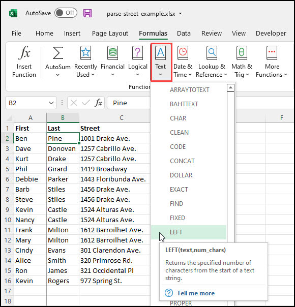
If you open this list in Excel and sort on the Street column, you get a numerically sorted list. As you can see in the example below, the Drake Ave records are not together. Our volunteers would go all over town based on this sort.

Ideally, you want to sort the list so the Drake Ave. entries are together. There are several ways to do this in Excel, but one way is to create two columns from the original alphanumeric string. You can’t easily extract text using Excel Text to Columns wizard since we have repeating delimiters.
The first column reflects the street number substring, and the second is the street name substring. You can then sort the list based on the street name and number.
Microsoft 365 Extract Text Functions
One benefit to using Microsoft 365, is it has additional functionality. If you have this subscription, then I would start with TEXTBEFORE and TEXTAFTER. Both these functions make it easy to extract text from a cell. They are the easiest and don’t suffer from some flash fill quirkiness.
Use TEXTBEFORE to Grab Street Number
The TEXTBEFORE function is true to its name. It grabs the contents of a cell before a specific delimiter. In our case, we’ll be using the space between the street number and the street name.
- Open your spreadsheet or use the sample spreadsheet in the Resource section.
- In cell D1, type NBR.
- In cell E1, type STREET NAME
- In cell D2, type the following formula:
=TEXTBEFORE(C2, " ",1,1)

With this formula, I’m asking Excel to extract the text before the space in cell C2. The first 1 represents the “instance number” of the delimiter. In my scenario, I want the first space. However, if I change the value to 2, the function would extract 1001 Drake because it would use the space between Drake and Ave. The second 1 in the formula indicates the match mode. The 1 is for case insensitive.
TEXTAFTER to Grab Remainder
You can think of TEXTAFTER as the compliment to TEXTBEFORE. The function works similarly except it extracts part of the text after your delimiter. In our scenario, we want to extract everything past the first space between the number and street name.
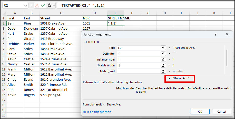
=TEXTAFTER(C2," ",1,1)
If you get confused with any of the parameters, you can always use the option of adding parameters using the Function Arguments dialog box. The dialog is nice since it provides context and highlights the result.

Building a Nested Extract Formula
For those that don’t have Microsoft 365,, we’ll nest some Excel functions such as LEFT and FIND. As we progress, we’ll add several sets of parentheses. By nested, I mean we’ll use one function (FIND) as an argument for another function, such as LEFT or RIGHT.
Using the FIND Function
Let’s start with =FIND(" ",C2). In plain text, our function syntax asks Excel to look in cell reference C2 for a single space represented by the “. ” I added a starting position of “1” in the picture below, but this is an optional parameter, and Excel starts at 1 by default. Excel found the blank space in position 5, which is shown in cell D2.

I’ll remove the optional starting parameter of 1 to simplify the formula since Excel starts there anyway.
In this scenario, I used FIND, which is case-sensitive. Microsoft has a SEARCH function, which is case-insensitive.
Using the LEFT Function
Now, let’s add the LEFT function so that our formula reads =LEFT(C2,(FIND(" ",C2))). In this instance, we’re again using cell C2, but the LEFT function will grab the cell contents in C2 from the leftmost character in position 1 to where the Excel FIND function found the blank space.

However, there is a minor issue. While you can’t see it, there is a trailing space in D2. Using the LEN function, we can see cell D2 has 5 characters. You may remember this handy function from our tutorial on how to check the character count in Excel.

The solution is to subtract 1 or use the TRIM function I referenced in how to separate names in Excel. For simplicity, I’ll use the -1. While the visual results are the same, the character count dropped by 1.

How to Extract Street Numbers Using LEFT Function
- Import your data into Microsoft Excel or use the sample spreadsheet in the Resource section.
- In cell D1, type Nbr.
- In cell E1, type Street Name
- In cell D2, type the following formula:
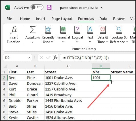
=LEFT(C2,(FIND(" ",C2)-1))
- Press Enter. The value 1001 should show in D2.
The next part involves copying this formula to the rest of the entries. First, we must reference the correct street cell and not use C2 for the remaining rows.
- Click cell D2 to select the beginning of our range.
- Move your mouse to the lower right corner.

- Double-click the + cursor in the lower right. This will copy your formula down the column.
In column D, you should see the extracted street numbers.
How to Extract Street Names Using the RIGHT Function
Using the RIGHT function, we’ll create a similar nested formula to capture the street address. This time, we will grab the contents from the Street column to the right of the first space.
- In cell E2, type the following formula
=RIGHT(C2,LEN(C2)-FIND(" ",C2))
- Press Enter. E2 should show as Drake Ave.
- Click cell E2 to select the beginning of our range.
- Move your mouse to the lower right corner.
- Double-click the + cursor in the lower right. This will copy your formula down the column.
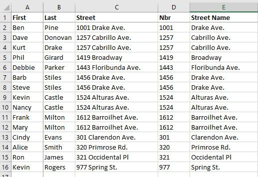
Columns D and E should contain the parsed contents from your original street address.
Your spreadsheet should look similar to the one below.

The spreadsheet now has your split fields, but you may want clean up the formulas. For example you might want copy formula values in Excel to values.
These Excel formulas to extract text from cell are key skills for efficient data management. They can simplify the process of sorting and analyzing spreadsheet data. Utilizing these functions effectively can lead to more productive and organized data handling. While we focused on using a space as our delimiter, they can be modified to handle your scenarios. Now, it’s your turn to practice.
