Use Excel Conditional Formatting to Highlight Cells

Have you ever stared at a spreadsheet looking for the important stuff?  The problem with many spreadsheets is that all the cells look the same. So you have to hunt for key or actionable information. In this tutorial, I’ll show how to highlight cells in Excel using built-in conditional formatting criteria. (Includes practice file.)

I routinely see this scenario. You get a spreadsheet from someone with hundreds of data rows that look the same. Everything is formatted in the same boring way. But is the data the same? Are there cell values that are different from the rest? Is something outside the average? These are typical questions users have when they open spreadsheets.

What is Conditional Formatting in Excel?

Instead of having the reader scan each cell, you can have Microsoft Excel do some legwork using some rules. This allows Excel to apply a defined format to a range of cells that meet specific criteria or conditions. These defined rules evaluate a cell value to see if it meets a specific criteria. If the condition is met, certain formatting is applied to the cell.

The goal is to make important information stand out so you can find it easier.

Excel already does some of this for you. For example, when you format numbers, there are options to display negative numbers in red. This is an example of a predefined format.

The program even allows you to use formatting options on individual cells or rows. The simplest method is to have Excel apply conditional formatting if it meets certain conditions or locations. This uses the “Cell Value Is” method.

Cell Value Highlight Examples

Below is a small sampling of ideas for using conditional formatting:

• Apply a red background fill if the cell value is less than 50
• Apply an italic, bold font style if the cell value is between 70 and 90
• Apply a green font color if the cell text contains “Montana.”
• Highlight cells that are equal to 15 with a red border
• Apply a yellow background fill to duplicate values
• Add an Up arrow icon to cell values above 10%
• Highlight all blank cells

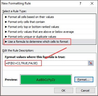
Excel also allows you to use formulas for conditional formatting. One benefit to Excel formulas is that you can reference the values elsewhere in your spreadsheet. In the example below, I’m using an Excel IF formula to test if the cell value in B2 is greater than the value in C2. If the formula is TRUE, apply a green background color.

Microsoft has greatly enhanced this feature over the years and now predefines popular examples, so you don’t need to rely on formulas as much. Below are some popular examples.

How to Apply Excel Conditional Formatting

Adding a new format rule is easy. The hardest part is finding what you want to highlight on your spreadsheet. It helps to think about your audiences’ needs and what actions they might take.

How to Highlight Cells Above a Specific Number

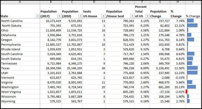
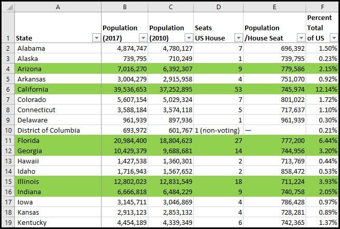
If you wish to follow along, this is Example 1 from the sample worksheet below. Again, I’m going to highlight selected cells if the state’s population exceeds or equals 2% of the US population.

1. Open the state-counts-cf.xlsx sample spreadsheet and click the Example 1 tab.
2. Click cell F2.
3. Select the whole column by pressing Ctrl +Shift + ↓.
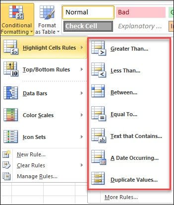
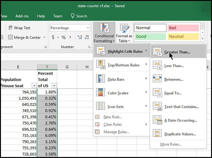
4. From the Home tab, click the Conditional Formatting button.
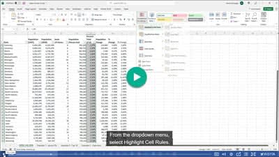
5. From the drop-down menu, select Highlight Cell Rules.
6. From the side menu, select Greater Than…

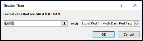
7. Adjust the value in the Format cells that are GREATER THAN: field.

Note: Excel will pre-populate this field based on the existing values of your highlighted cells.

8. Enter your desired value. In our case, it’s 2.0%. Excel will start highlighting cells for you.
9. Click the down triangle ▼ to make your color selection.

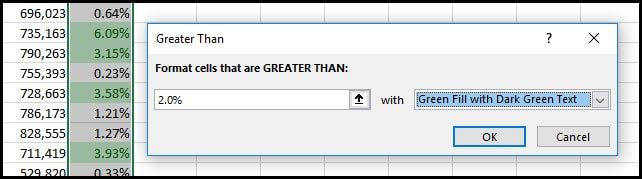
✪ Note: You can create a different color scheme by selecting a Custom Format.

10. Click OK.

You should now see your results applied.

How to Highlight Top 10 Items

One popular request is to find the top entries, whether they be a set number or percentage. This is an example of one of Excel’s preset or built-in formats. In other words, you don’t need to enter specific values as you did in Example 1. Instead, these presets are built around common items people look for, such as Top 10 or below-average performers. The advantage is that you don’t have to do the math.

In this example, I want to highlight the top 10 states by US House Seats in Column D.

1. Open the state-counts-cf.xlsx sample spreadsheet and click the Example 2 tab.
2. Click cell D2.
3. Select the whole column by pressing Ctrl +Shift + ↓.
4. From the Home tab, click the Conditional Formatting button.
5. From the Conditional Formatting drop-down menu, select Top/Bottom Rules.
6. From the side menu, select Top 10 Items…
7. In the Top 10 Items dialog box, adjust your count or color scheme if necessary.
8. Click OK.

One advantage to using color is that Excel can sort by color too. Additionally, you can also SUM or COUNT colored cells.

How to Use Data Bars Instead of Background Color

Another useful option is to use “Data bars.” This is another type of visualization that you can apply. A key difference with the Data Bar format is that it shows all cells instead of those meeting a specific condition.

By default, Excel will keep the text value background. I find that this can be distracting. In this example, I duplicated the % Change column but told Excel not to put the data value in Column I. The result is just the data bar.

The data bar format doesn’t work well with all data types. This is a good example of trying different formats to see what works best for your data. This is especially true if you have negative values or a tight range.

1. Open the state-counts-cf.xlsx sample spreadsheet and click the Example 3 tab.
2. Click cell I2.
3. Select the whole column by pressing Ctrl +Shift + ↓.
4. From the Home tab, click the Conditional Formatting button.
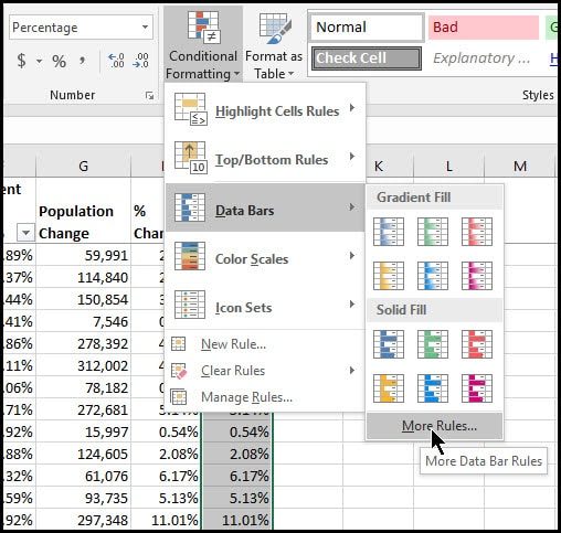
5. From the Conditional Formatting drop-down list, select Data Bars.
6. From the side menu, select More Rules…

7. In the Edit the Rule Description: section, check Show Bar Only.

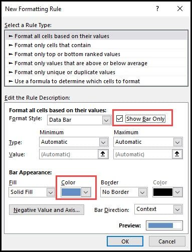
8. Click OK.

How to Highlight a Row

Highlighting outlier cells is great, but sometimes if you have a large spreadsheet, you may not see the colored cells because they’re off-screen. In these situations, it helps to highlight the entire row. That way, regardless of which columns you’re viewing, you know which rows are important. This works best when you have 1 conditional.

A key difference here is we won’t be highlighting a column but the entire spreadsheet. That’s how we get the row effect.

1. Open the state-counts-cf.xlsx sample spreadsheet and click the Example 4 tab.
2. Click cell I2.
3. Select all rows by pressing Ctrl +Shift + ↓ + ←.
4. From the Home tab, click the Conditional Formatting button.
5. Select New Rule…
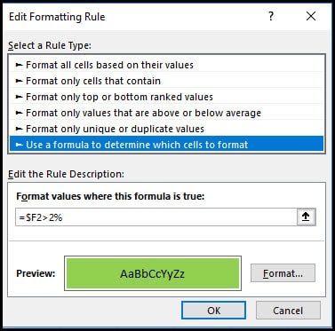
6. In the Edit Formatting Rule dialog box, select Use a formula to determine which cells to format.
7. In the Format values where this formula is true: type your criteria.

8. Click the Format button to apply your highlight color.
9. Click the Fill tab.
10. Select your color.
11. Click OK to accept your color.
12. Click OK to close the dialog box.

In the example above, I want to highlight any row where the value in column F (Percent total of US population) is greater than 2%. The highlight color is green. I’m also using a mixed cell reference by placing a $ sign before F2 in the formula.

✪ Tip: If you’re not sure you have the correct formula, you can always test it in another column. For example, I could enter in cell H2, this formula =$F2>20%. The H2 cell would be evaluated as either TRUE or FALSE. You could then copy the formula down the column to make sure you get your expected results.

13. Click OK.

Find Existing Conditional Formating Rules

Sometimes we’re given a spreadsheet, and you see highlighted cells or rows. But… where are the conditional rules, or did someone manually format these cells? Fortunately, Excel provides a way to see conditional formatting rules. You can use the example spreadsheet to follow along or use your own.

1. Open up your spreadsheet.
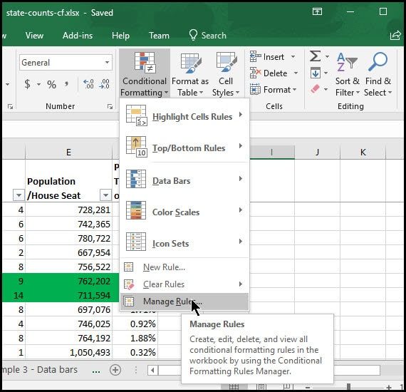
2. From the Home tab, click Conditional Formatting.
3. Select Manage Rules… from the drop-down list.

4. In the Conditional Formatting Rules Manager dialog box, select your worksheet.
5. Click OK.

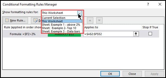
In the example above, you can see the rule I applied to highlight the row. From here, you could add a rule, edit the rule, or delete it.

Highlighting Tips & Tricks

This tutorial touched on some of the ways you can use conditional formatting to highlight cell values. The best way to learn is to experiment with some data, whether it’s your own or the sample spreadsheet. Here are some other tips for you:

• You can have multiple rules in the same column. For example, you might want to have different range values, be different colors.
• Play around with different formats to see which type works best for your data.
• If you get unexpected results, check to see if multiple conditions are being run and the rule order. You may need to change the order.
• You can set ranges on data bars. For example, if you have a % Complete column, you may want to set a range of 0 to 1.
• You can remove conditional formatting rules with the Clear Rules option.
• Apply your rules after you’ve entered data. Sometimes duplicate rules are created when you insert rows.

Excel’s conditional formatting can make your spreadsheets more useful if used appropriately. People won’t waste time looking for important changes or that “needle in the haystack.” Play around and create your own custom cell styles and conditional formats.

Show Me How Video

To see the above examples, click the image below to be taken to the accompanying video and transcript.

Excel Practice File

Hand-picked Excel Tutorials

• Beginners Guide to Excel XLOOKUP
• How to Use Excel VLOOKUP
• How to Check Excel Cells for Specific Text
• How to Use Flash Fill in Excel
• How to Create an Excel Pivot Table