Have you ever wanted to group or filter cells in your Excel spreadsheet based on the cell background or font color? In this tutorial I’ll show you how to use this powerful feature to organize, analyze, and visualize your data. See how this simple technique can increase your productivity and improve data analysis. (Includes practice file.)
Knowledge You Will Gain
- Understand the benefits of sorting and filtering by color in Excel.
- Learn how to sort data by cell color, font color, and conditionally formatted colors.
- Master the steps to filter data based on color.
- Discover techniques for handling potential errors or limitations.
- Find a font’s RGB color value.
Benefits of Sorting and Filtering by Color
The tutorial below can be used for font colors or cell background colors. Some people may refer to these as highlighted cells. For these instructions, I’ll be using Microsoft Office 365. However, these steps can be used in stand-alone Excel versions.
It’s probably my laziness, but changing a cell’s background or text color is useful. Here are some of the benefits I’ve experienced:
- Improved visuals – color stands out and draws the eye
- Faster data analysis – color lets you focus on important data points or highlighted cells
- Faster workflows and automations when using conditional formatting
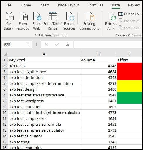
I’ve already built a sample spreadsheet with some values and colored cells. Please don’t put any value in the data as it’s for illustration. I used a keyword generator and Excel’s randbetween function to create it.
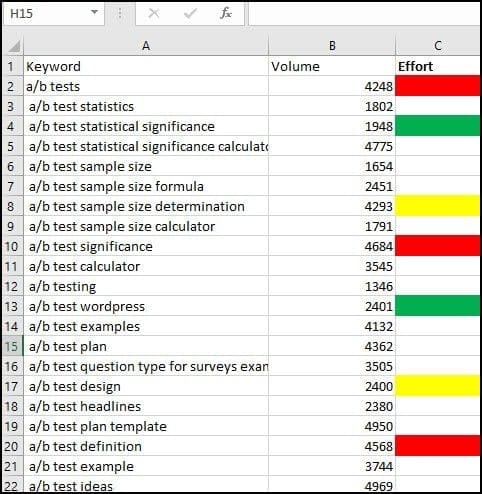
I’ve applied the cell background color to Column C in my screen snap above. However, some people might prefer using color across a row. In the second screenshot below, I used Excel conditional formatting. The process is the same regardless of whether you’re using columns or rows. It also works with Excel tables.

How to Sort by Cell Color
- Open your spreadsheet and click the Data tab.
- Highlight your data range. You can also click CTRL + Shift + → + ↓.
- Click the Sort button.
- Tick the My data has headers checkbox in the top-right if your worksheet uses them.
- Click the + Add Level button.
- Click the drop-down arrow next to Sort by ▼ and select the column label with your color.
- Move to the right and click the drop-down arrow for Sort On values.
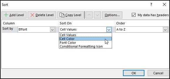
- From the drop-down list, select Cell Color. Excel will show the colors you used from the spreadsheet including “No cell color”.
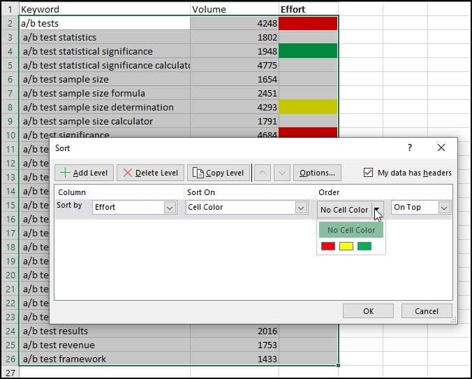
- Select your first fill color and keep the Order value as On Top.
- Click the Add Level button in the top left of the panel. This will add another sort order rule.
- Add in your other color levels. If you prefer, you can also use the On Bottom option.
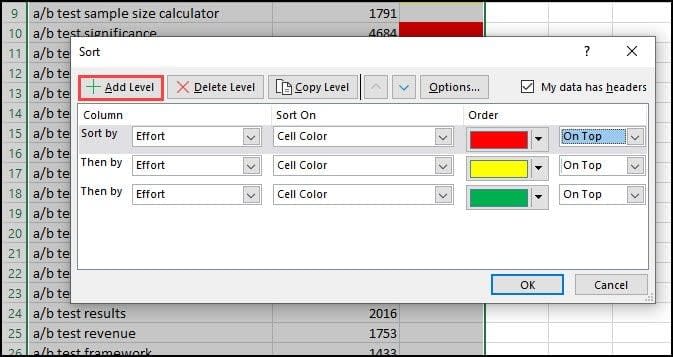
- Click OK.
You should now see your list sorted by color. You’re not limited to 3 colors; you can keep adding if they’re on your sheet. You also don’t need to enter the last color, as Excel will put it on the bottom. In my case, that was “No Cell Color.”
How to Sort Data by Font Color
The process of sorting by font color is similar to the steps above. However, there is one additional sorting option called “Automatic“. I’m not in love with the name, but Microsoft doesn’t give me a vote.
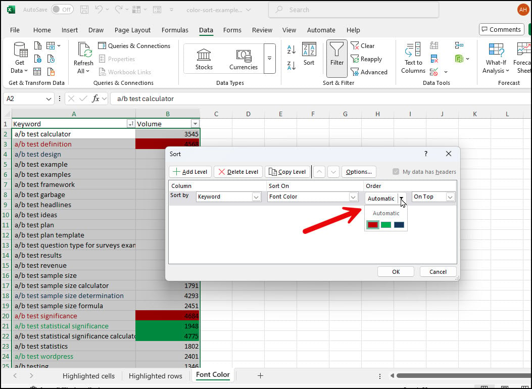
If you’re like me, you wondered what “automatic” meant. At first I thought it was sorting by the order the color appeared on the spreadsheet. No, it is using the font color’s RGB value. I question the value of this option, but some people may need it.
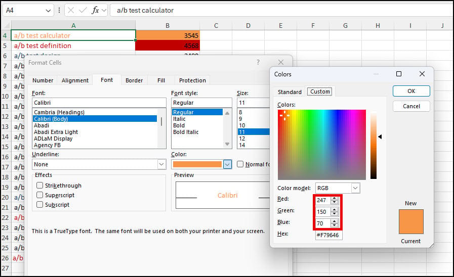
Finding a Font RGB Color
- Click in the desired cell.
- Right-click and select Format Cells.
- Click the Font Tab.
- Click the color drop-down menu and select More Colors.
- On the Colors dialog, click the Custom tab.
- The RGB values will show under the Color model section.
How to Filter by Cell Color in Excel
Some people prefer to filter instead of sort. This is great if you want to focus on certain items, maybe overdue invoices. Even better, the procedure is shorter.
- Open your spreadsheet.
- Select the column you wish to filter that has color.
- From the Sort & Filter group, click the Filter button. You should see a small drop-down arrow in the top-right corner of your column heading.
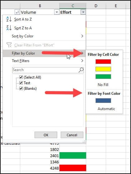
- Click the down arrow ▼ and select Filter by Color.
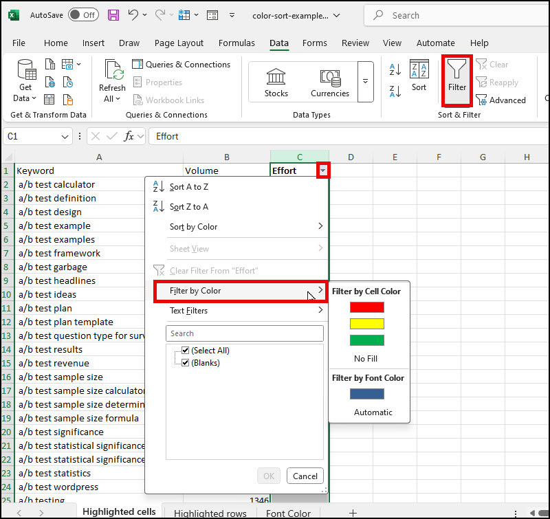
- Select your cell color from the side menu.
In my example, I was using a cell color. However, when I added colored text, Excel adjusted the options. On the side menu for Filter by Color, you would also see Filter by Font Color.
Quick Takeaways
- Excel allows you to sort and filter by color.
- The color can be either the cell background color or the font color.
- You can place colors on top or bottom.
- The system knows which colors you’ve used.
- You can add multiple color sorts.
- Sort rules are processed in order
As we’ve seen, sorting and filtering by color in Excel are useful techniques that can improve your data analysis. By learning these simple yet powerful features, you can find trends, group similar data points, and extract meaningful insights from your workbook.
Below you’ll find a practice file containing three sheets with various color options. Why not start practicing your color sorting and filtering skills? With a little practice, you’ll be able to harness the full potential of color-coding. For example, did you know you can sum colored cells in Excel?
