Ever find yourself repeatedly scrolling to see which spreadsheet column or row you’re working on? Excel sticky headers are your solution. This feature lets you lock any combination of top rows and left columns in place, ensuring they remain visible no matter how far you scroll down or across your data. Discover four ways to customize this feature. Enhance your productivity by keeping key data in sight and streamlining your navigation.
Knowledge You’ll Gain
- Understand the functionality of freezing versus splitting panes for better data management.
- Discover how to lock specific rows and columns to suit your viewing needs.
- Gain quick access to freeze and split pane functions with handy keyboard shortcuts.
- See common reasons why freeze panes may not work.
Understanding Excel Panes: Locking Your Data In View
An Excel pane is a set of columns and rows defined by cells. You get to determine the size, shape, and location. For many people, it might be the top row. This is sometimes called a “sticky header” since it stays in the same location. For others, it’s an inverted L-shape and contains the top row and first column. You’re the spreadsheet architect and can define your pane.
Regarding spreadsheets, you can “freeze panes” or “split panes.” Splitting panes is a bit more complex because you have separate windows of your data on the worksheet. So, for the sake of simplicity, this tutorial will cover freezing panes.
If your columns and rows aren’t in the orientation you want, you may want to learn how to transpose or switch columns and rows in Excel.
TextExpander: Worth It? Find Out.
Is TextExpander the right tool to boost your productivity? Get an independent assessment, weigh the pros and cons, and make an informed decision. Find out why I’m a fan.
Read the ReviewWhy Lock Columns or Spreadsheet Cells?
A key benefit to locking or freezing cells is seeing the important information regardless of scrolling. The split pane data stays fixed or “sticky”. Your spreadsheet can contain panes with column headings, multiple rows, multiple columns, or both.
Otherwise, losing focus on a large worksheet is easy when you don’t have column headings or identifiers. I’ve had times where I’ve entered data only to find I was one cell off and produced Excel formula errors. By locking various sections, you have a consistent reference point. This also helps readability.
Typically, the cells you want to stay sticky are labels like headers. However, they could just as easily be an entire column, such as employee names.
Let’s go through four examples and keyboard shortcuts to freeze panes in Excel.
1 – How to Freeze Top Row in Excel (Sticky Header)
This freeze row example is perhaps the most common because people like to lock the top row that contains headers, such as in the example below. Some people also call this a “floating header” because it always floats to the top as you scroll down.
Another solution is to format the spreadsheet as an Excel table.

- Open your worksheet.
- Click the View tab on the ribbon.
- Click the small triangle ▼ (drop-down arrow) in the lower right corner of the Freeze Panes button. You should see a new menu with three options. Note the icons as they provide visual clues.

- Click the menu option Freeze Top Row.
- Scroll down your sheet to ensure the first row stays locked at the top.
You should see a darker border under row 1.
Keyboard Shortcut – Lock Top Row
I like to do this shortcut slowly the first time to see the ALT key letter assignments as you type. I can see the keyboard assignments in the example below once I hit my Alt key. Some people prefer to add the Freeze Panes command to the Quick Access toolbar because they frequently use it.

Alt + w + f + r
2 – How to Freeze First Column
A similar scenario is when you want to freeze the leftmost column. I find this option helpful when I have a spreadsheet with many columns and I need to fill in data without using an Excel data form.
- Open your Excel worksheet.
- Click the View tab on the ribbon.
- On the Freeze Panes button, click the small triangle ▼. You should see a new menu with your 3 options.
- Click the option Freeze First Column.
- Scroll across your sheet to ensure the left column stays fixed.
Keyboard Shortcut – Lock First Column
Alt + w + f + c
Science-Based Focus Music Tested
Brain.fm creates functional music specifically engineered to enhance your concentration. Backed by NSF-funded research and proven with EEG studies. Learn how their specialized audio patterns help you maintain peak mental performance.
Read Our Review3 – How to Freeze Top Row & First Column

This is my favorite option. If you look at Microsoft’s initial Freeze Panes options, there isn’t one labeled “top row and first column”. However, if you look at the icon you can see it visually matches Freeze Panes.
The subtext reads, “Keep rows and columns visible while the rest of the worksheet scrolls (based on current selection).” Some folks get confused as they think they have to highlight data to make a selection.
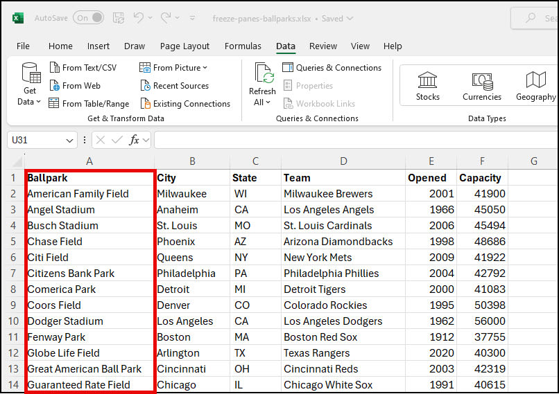
Instead, consider the selection of the first cell outside your fixed column and row. If I wanted to lock the top row and top column, that selection cell would be cell B2 or Milwaukee. Regardless of whether I scroll down or to the right, the first cell that disappears when I scroll is B2.

- Open your Excel spreadsheet.
- Click cell B2. (Your set cell.)
- Click the View tab on the ribbon.
- On the Freeze Panes button, click the small triangle ▼ in the lower right corner. You should see a dropdown menu with your 3 options.
- Click the option Freeze Panes.
- Scroll down your worksheet to ensure the first row stays at the top.
- Scroll across your sheet to ensure your first column stays locked on the left.
Keyboard Shortcut – Freeze Panes
Alt + w + f + f
4 – Freeze Multiple Columns or Rows
Occasionally, I get Excel worksheets where the author puts descriptive text above the data. My header isn’t in Row 1 but further down in Row 5. Or, I want to lock multiple columns to the left. I want to lock Columns A & B and Rows 1-5 in the example below.

The process is the same, I need to click the set cell that stops the fixed area. In this case, it would be cell C6 or “Chase Field.” The content above and to the left is frozen.
Everything in the red boxes would be locked. The downside is you may give up much of the screen real estate.
Why Freeze Panes May Not Work
There are some rules surrounding this feature. If you don’t follow these, freeze panes may not work.
Quick test: If you type Ctrl + Home and your cursor moves to cell A1, you haven’t locked anything.
- If you dislike your settings, use the Unfreeze Panes command.
- This feature won’t work on a protected worksheet or Page Layout View.
- If you edit a value in the Formula bar, the View menu will be disabled.
Microsoft has instructions for seeing the same header on printed pages.
Mastering Excel panes and floating headers can enhance your ability to manage large spreadsheets, ensuring a more efficient workflow. If you enjoyed this tutorial and want to boost your Excel skills further, check out the hand-picked Excel tutorials below. Each tutorial is designed to help you become more proficient and confident in handling various Excel functions.