Ever wondered how to boost productivity while using Excel? Get to know the Excel ribbon, the one-stop destination for shortcuts and commands. For example, it hides part of the toolbar when I need more space or want to be in distraction mode. In this tutorial, I’ll show you how to customize the Excel ribbon by adding more features, such as the Developer tab.
What is the Excel Ribbon
Microsoft introduced the ribbon with Office 2007. It replaced menus and toolbars with a new interface with the same functionality. Within the toolbar, you have contextual elements:
- Tabs – these are major divisions that run along the top. (e.g., Data)
- Groups – these are similar items within a Tab. (e.g., Get & Transform Data)
- Commands – these are features within a Group represented by a button. (e.g., Filter)

All tabs have the above elements. However, some tabs, such as Page Layout, have another called the Dialog Box Launcher. When present, it is in the lower right corner of the Group. When clicked, it will open an additional dialog like Page Setup.
When Excel is set up, it contains the following ribbon tabs:
- File
- Home
- Insert
- Draw
- Page Layout
- Formulas
- Data
- Review
- Help

TextExpander: Worth It? Find Out.
Is TextExpander the right tool to boost your productivity? Get an independent assessment, weigh the pros and cons, and make an informed decision. Find out why I’m a fan.
Read the ReviewShow and Hide Ribbon Elements
For most people, the ribbon shows under the Quick Access toolbar. Sometimes you don’t see the Excel ribbon because it is hidden. It’s not missing but in a “collapsed” state. Some prefer closing it to have more room to work on the spreadsheet.

How to Collapse the Excel Ribbon – Method 1
The process for opening or collapsing the menu is the same. The only difference is the menu may show a checkmark to reflect your current state.
- Place your mouse over any ribbon tab name. (e.g., Data)
- Right-click and select Collapse the Ribbon.
Keyboard shortcut: Ctrl + F1

Show or Hide Using Ribbon Display Options – Method 2
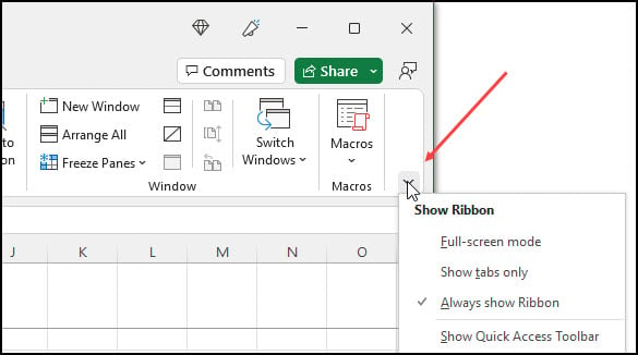
Anyone around Microsoft products knows there are multiple ways to do tasks. For example, looking at your Excel sheet’s top right, you’ll see a small icon before the minimize button. It’s squarish and has an upwards arrow. This is for the Ribbon Display Options. In some cases, this button may be easier to use.
If you click the button, you’ll get three options:

On Microsoft 365, the menu option has moved to the lower right corner of the ribbon.

The items are pretty self-explanatory. The one caveat is that clicking Auto-hide Ribbon will also make your spreadsheet fill your screen.
How to Reopen a Collapsed Tab
When you collapse the ribbon, all you’re doing is temporarily hiding the groups and commands. The tab names are still showing much like a menu. To bring back these items, click the Tab. Your groups and commands will reappear. When you’re done, click the Tab again, and it will collapse.
Add Excel Developer Tab & Other Tabs
When you first install Excel, it doesn’t enable all the tabs and commands. Microsoft tends to put in the frequently used ones and allows users to add the rest. The Developer tab is one of the first ones people like to add back in. This is very handy if you use Excel macros as this Contextures tutorial illustrates.
- Place your mouse over any tab name. (e.g., Data)
- Right-click and select Customize the Ribbon….
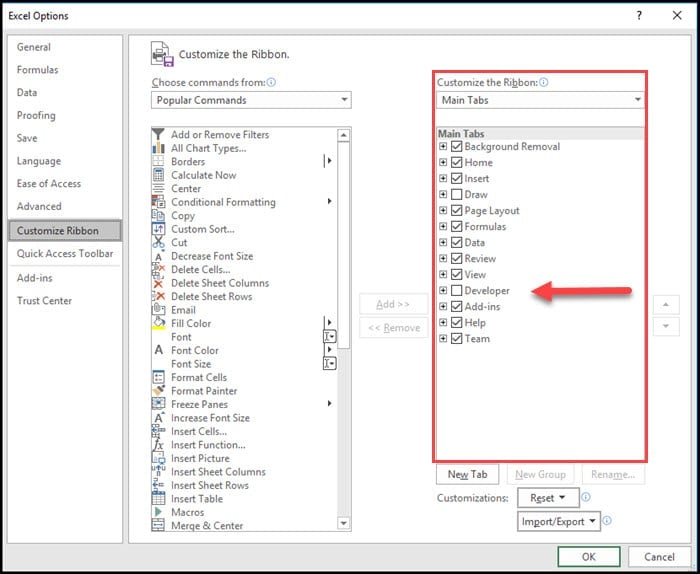
The Excel Options dialog will open.
- From the Customize the Ribbon: section on the right, check the box for Developer or another Tab.

If you don’t see your Tab, change the drop-down menu on the top of the right panel from Main Tabs to All Tabs.
- Click OK.
The Commands and Ribbon Structure
When adding commands, it helps if you remember the ribbon’s hierarchy. While adding a command to the ribbon, we’re adding it to a custom group within a tab. Commands aren’t standalone, and you can’t shoehorn them into an existing group. If you try to add an unused command to an existing group, you’ll get a Ribbon Customization error message that reads:
Commands need to be added to custom groups. To create a group, pick a tab in the list, then click New Group.
There is another Excel option. Commands that aren’t displayed by default have to go in a “custom group.” You can choose to have this custom group on an existing tab or create a custom tab.

How to Add a Command
- Place your mouse over any tab name. (e.g., Data)
- Right-click and select Customize the Ribbon….
The Excel Options dialog will open.
- Under the Choose commands from: drop-down menu, select Commands Not in the Ribbon.
- Scroll down the list and click the command you wish to add. (e.g., Form…)
- Decide whether the Command will go on an existing tab (e.g., Formulas or new tab.
I prefer to create a new tab because many of the default Tabs are full.
- From the right side, click the New Tab button toward the bottom.
Under the Main Tabs section, you should now see New Tab (Custom) and New Group (Custom).
The item should also be shaded. The shading indicates this section will be accepting the new command.

- Click the Add >> button in the center.
We need to rename our New Tab (Custom) and New Group (Custom).
- Click to highlight the New Tab (Custom) item.
- Click the Rename… button.
- Provide your new Tab name. (e.g., Custom, My Stuff)
- Click OK.
- Repeat the rename process for New Group (Custom).
Save Excel Ribbon Configuration
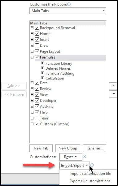
If you’ve made many customizations to your ribbon or are fearful some other user might change it, you can export your ribbon settings. This will produce an Excel Customizations.exportedUI file.

You can then import that file back into Excel. It will overwrite your existing settings. However, you will not see your changes till you click the final OK.
Now that we’ve unraveled Excel ribbon customization, you’re on your way to a more personalized and productive Excel experience. But don’t stop here. Have you tried freezing panes to make a sticky header? There’s a world of possibilities waiting to be explored in Excel. Keep experimenting, keep learning, and most importantly, keep customizing.
