Have you ever struggled to find and link specific information in your Excel spreadsheets? VLOOKUP is a powerful function available to all Excel users that helps you extract data based on specific criteria. In this beginner’s guide, I’ll show how to use VLOOKUP effectively using two examples to bolster your data analysis skills. Includes practice file and video tutorial.
Knowledge You’ll Gain:
- How to use VLOOKUP to find specific information within your Excel spreadsheets.
- Understand the key components such as lookup values, table arrays, and column index numbers.
- Apply VLOOKUP to real-world scenarios, such as extracting data from different tables or using the included practice file.
- Troubleshoot common VLOOKUP errors and resolve issues effectively.
- Develop a solid foundation for exploring more advanced Excel functions and techniques.
Trial By Fire
When I first heard about this powerful Excel function in 2005, I looked at the help file and syntax. I then rolled my eyes.
VLOOKUP(lookup_value,table_array,col_index_num,[range_lookup])
It didn’t look easy, and I couldn’t see the immediate benefit. But sometimes, pushing through difficulties can make things easier in the long run. I’m glad I did because it helped me with some huge voter data files.
If you’re using Google Sheets, please see Using Google Sheets & VLOOKUP.
I like to start with an easy example when learning Microsoft Excel formulas and functions. This VLOOKUP tutorial will provide two examples using different function arguments and lookup values.
- Example 1 uses one worksheet with an Approximate match. You’ll be referencing a table on the existing sheet.
- Example 2 uses two worksheets with an Exact match. You’ll be referencing data from another worksheet.
Understanding Excel’s VLOOKUP Function
VLOOKUP is an Excel function that allows you to search and retrieve a cell’s content from one column and use it in another location to retrieve data. As you might guess, the “V” stands for vertical and relies on looking up data from a lookup table column.
This lookup column could be on the same worksheet you’re viewing or another within your workbook. The function requires a common field or key and four arguments. In addition, the function allows you to specify whether to use an exact match or an approximate match.
Why Use a VLOOKUP Formula?
Let’s put these terms in context and give an example of how the function might be used. It’s similar to one of the practice exercises. When I was working on our local elections, the county provided a massive file with the data. Each worksheet contained info I might use.
The problem is I had numerous worksheets in this workbook. I didn’t want to switch between each sheet. That’s not efficient. Moreover, I wanted to do some of my own calculations using other Excel formulas.
The solution was to find a common denominator or key between these worksheets. Using this common key, I can create a new worksheet and pull the needed columns from each worksheet using the VLOOKUP function. Again, Microsoft Excel does the heavy lifting. This allows me to concentrate on one worksheet with the data I need.
You might have your own examples, such as retrieving data using a shopkeeping unit (SKU) or ISBN if you deal with books, part numbers, etc.
VLOOKUP Example: Approximate Match
The example outlined here is found on the Example 1 worksheet, which can be downloaded at the end of the tutorial. All the names are fictitious.
One cell reference contains the voter’s birth date. However, I didn’t want the voter’s birth date to show on the final distributed files. But, I did want to do some age analysis.
Instead, I created a segment based on age ranges and a lookup formula. Excel would do a vertical lookup that returns the matching value from one column to the desired cell. For example, rather than showing a voter was 28, I would define them as “Young.”

Let’s refer to the screenshot above with my first voter, Sophia Collins. If you scan Column D (Age), you’ll see she is 43 years old and in the “Mature” Segment. This is because the value of “Mature” in Column E was dynamically pulled using Excel’s VLOOKUP function.
The lookup table in Columns H and I with blue headings is the small Excel table. Microsoft refers to this as a table_array. This is where I’ve defined my four age segments: New, Young, Mature, and Senior.
My “Segment” works because if a voter is under 21, they are “New.” From 21-38, they are “Young.” From 39-59, they are “Mature.” And if they are 60 or older, they are “Senior.”
In Sophia’s case, Excel would take her age of 43 from cell D2 and return the closest match from Column H. Both columns D and H contain age data, which is our standard key.
When Excel found an approximate match, it would go to Column I and get the Label. The returned value of “Mature” was then copied to cell E2, the Segment.
You might notice that the lookup table doesn’t list every age. It doesn’t have to because I’m using an approximate match. I’m telling Excel to find me the closest age.
For example, the next voter Evelyn Bennett is 54, but there is no value for 54 in Column H. In this case, 54 falls between 39 and 59, so she is also labeled “Mature.”
As we stated, to use the VLOOKUP function, there needs to be a common key. In this case, it’s age. Both columns D and H contain ages. The column headings and cell contents can be different and don’t have to be an exact match.
Learning VLOOKUP Arguments
Let’s peel away some of the mystery and display how VLOOKUP shows in the Excel formula bar. In this illustration, I’ve clicked cell D2.
The term “argument” isn’t as complicated or negative as it sounds. If you’re familiar with the Excel formula bar, an argument is what goes in between the parentheses ( ). It provides an input value for the Excel function.

[A] – This represents the VLOOKUP formula in Cell E2.
=VLOOKUP(D2,$H$2:I$5,2,TRUE)
[B] – Cell D2 is our first argument called Lookup_value.
[C] – The cell range $H2$2:$I$5 is our Table_array and the second argument.
[D] – 2 is the Col_index_num from our Table_array and the third argument. Label is the 2nd column.
[E] – TRUE is the Range_lookup and the fourth argument.
The good news is the VLOOKUP Function Arguments dialog box guides you through these elements, so you don’t need to type the long string in Excel’s formula bar.

VLOOKUP Arguments
Some functions have required arguments, while others don’t. For example, to compute the voter’s age, I also used the TODAY function =TODAY(), which doesn’t use any arguments. Some common argument examples include:
- cell range
- true/false logical value
- number
Using the formula from cell D2, here’s how these four arguments work.

1. Lookup_value – Think of this field as your starting point. Excel will look for a match to this value in the leftmost column of our table_array. In this example, I want to look up Sophia’s Age from cell D2.
2. Table_array – This is the cell range for your lookup table or where you want to search. This range lookup can be on your existing worksheet or another worksheet. For example, I have a small table with the age groupings and corresponding labels in this example.
3. Col_index_num – The column number on your lookup table with the necessary information or search results. In our example, we want column 2, which has the column heading of Label. This will be our voter’s Segment name.
When we count, we’re counting the columns on the lookup table. So even though the “Label” column is Column I or the 9th column, it’s the 2nd column on the lookup table. Some people call this a Column Index.
4. Range-lookup – this field defines how close a match should exist between your Lookup_value (D2) and the value in the leftmost column on our lookup table. In our case, we want an approximate match, so we’ll use “TRUE.”
VLOOKUP’s Table Array: Rules & Best Practices
There are several rules to remember about this table array.
For example, if I want to use the same formula in cells E3 through E11, I don’t want my lookup cell references to shift each time I move down to the next cell. I need the cell references to be constant. This is called an absolute cell reference.
After you define your lookup range of cells, you can press F4. This will cycle through absolute and relative cell references. You want to select the option that includes a $ before your Column and Row. You can get around this if you know how to create named ranges in Excel.
Step by Step: Adding VLOOKUP Formula
The steps below were used for Example 1 from the practice file.
- Add in the column where you’ll enter the VLOOKUP formula. In my case, I added Column E and called it Segment.
- Add in your lookup table and data. Mine is H1:I5.
- Click cell E2.
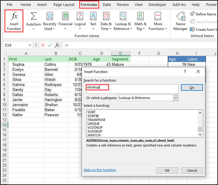
- Click the Formulas tab from the Excel ribbon.
- Click the Insert Function button.
- From the Insert Function dialog box, type “vlookup” in the Search for a function textbox. You may also select it from the Lookup & Reference category.
- Click Go.
- Click OK. The Function Arguments dialog box will appear with text boxes for the required arguments.

- In Lookup_value type D2. Or, you can click the cell.
- In Table_array type $H$2:$I$5. Note the $ signs.
- In Col_index_num type 2.
- In Range_lookup type true.
- Your Function Arguments dialog should look like the following. Notice in the lower left; you can see the Formula result.

- Click OK. You should now see “Mature” in cell E2.
- Click cell E2.
- Click the small green square (fill handle) in the cell’s lower right corner to copy the VLOOKUP formula down the column.

You might want to use the Excel formula auditing feature if you get any error messages.
Differences Between VLOOKUP and XLOOKUP
Now, you might have heard of another Excel lookup function called XLOOKUP. This function is available in Microsoft 365 subscriptions. However, if you’re using a standalone version like Excel 2016, you won’t have access to XLOOKUP.
Here are a few key differences between the functions:
- Search Direction: XLOOKUP can search left and right within a table. VLOOKUP can only search to the right of the lookup value.
- Column Changes: It’s easier to manage your data with XLOOKUP. It doesn’t rely on column index numbers like VLOOKUP. This makes adding or deleting columns easier.
- Default Match Type: XLOOKUP defaults to an exact match, which I use more often. VLOOKUP requires you to specify the match type explicitly.
VLOOKUP & Multiple Spreadsheets: Exact Match Example
The second scenario dealt with that same election file. This time there was an extra worksheet for political parties. The voter’s party was listed as an alphanumeric value called “Pcode” and not the political party.
This coding wasn’t intuitive. For example, “D” was for the “American Independent Party,” but some thought it meant “Democratic Party.” Another difference was we needed an exact match for the Political party.

Again, the way to solve this problem was to use the worksheet with the Pcode and translation and have Excel use the VLOOKUP function for the Party name. I could add a column called “Political Party” to my original worksheet to show the lookup table’s information.
Using the Starting VLOOKUP Practice File
- Download the practice file. The file link is at the bottom of this tutorial.
- Review Example 2 – Voters worksheet. It has the voter’s first and last names but only a Pcode.
- Review Example 2 -Party Codes worksheet. It has a listing of party codes and political names. Each of the Party Codes and Names is unique. You’ll also note that Column A is sorted in ascending order.

- Add your new column on the Voters worksheet that will display the info pulled from the Lookup table on the Party Codes worksheet. In my example, I added a column called Political Party in Column D. This is where I will insert the Excel function.

- Place your cursor in the first blank cell in that column. In my example, this is cell D2.
- Click the Formulas from the Excel ribbon.
- Click the Insert Function button.
- From the Insert Function dialog, type “vlookup” in the Search for a function textbox.
- Click Go.
Understanding VLOOKUP Arguments
After you click OK, Excel’s Function Arguments dialog appears and allows you to define the four values. You’ll see that your starting cell and the formula bar show the beginning part of the function =VLOOKUP(). The Function Arguments dialog adds the needed data elements that will display between ().
For illustration purposes, I overlaid the Party Codes worksheet to show the relationships.

After entering the required arguments, my dialog looks like the example below.
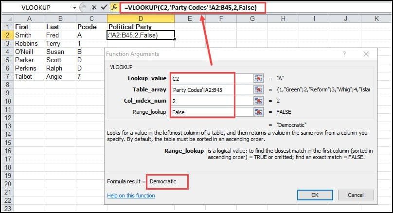
You can see this in the red outlined formula bar above. I now have more information based on my Function Arguments dialog box entries. You might also note that when I clicked the Party Codes worksheet to add in my Table_array, Excel prepended the worksheet name before the cell range. However, I must return and enter my $ signs to make the cell references absolute.
The other item of interest is that Excel displays the Formula result = text line when you build these functions. This is great feedback that can show if your function is on target. In our example, Excel looked up the Pcode of “A” and returned the Political Party “Democratic.”
VLOOKUP is a powerful Excel function that can leverage spreadsheet data from other sources. There are many ways you can benefit from this function. I used a 1:1 code translation in this example, but you could also use it for group assignments. For example, you could assign state codes to a region such as CT, VT, and MA to a “New England” region.
One important note about using Excel functions and formulas is you want to be careful when deleting columns.
For example, I omitted the Age column in the final spreadsheet I distributed. After completing my VLOOKUP and getting my segments, I copied the cell values to a new Excel worksheet. If I had just deleted Column D, my Excel formula would’ve returned an error.
If you’re trying to do a horizontal lookup, you’ll be happy to learn that Excel has an HLOOKUP function. I haven’t done an HLOOKUP tutorial yet. If this interests you, let me know. However, Microsoft has released a new versatile vlookup alternative function called XLOOKUP.
Troubleshooting and Errors
Before you grab the practice file below, you might want to review these points.
- If you get a #N/A error your lookup value wasn’t found in the first column of your lookup range. This could also be based on your match type. Maybe you have extra spaces or a data type mismatch.
- It’s important to use absolute cell references when defining your table array in VLOOKUP. This ensures the correct cells are referenced when the formula is copied to other cells.
- If you get a #REF error, you probably have a formula error. For example, your col_index_number is greater than the number of columns in your table_array
As this tutorial has shown, VLOOKUP is a powerful function that allows you to find and extract information, whether in one workbook or multiple. Download the practice file below and play around with the formulas and examples. See if you can recreate any of the errors above and fix them. You’ll be well on your way to improving your spreadsheet skills.