How to Use VLOOKUP Formula in Google Sheets

Have you ever dealt with a spreadsheet where you needed to look up a value that was someplace else? Maybe it was a part number, and you wanted to know its name. Google Sheets has a lookup function that can handle this. This function is popular among Google and Microsoft spreadsheet enthusiasts. In this tutorial, I’ll show how to apply VLOOKUP in Google Sheets. (Includes practice spreadsheet).

If you’re a Microsoft Excel user, please check out the Excel VLOOKUP tutorial.

What is a Lookup Function?

If we remove the spreadsheet concept, you probably do a similar lookup when you go to a restaurant. You scan the menu for items and prices. And just as you’re about to order, there’s a reference to “daily specials.” Now, you have to hunt for where the daily specials items are posted or ask. I often find them on a chalkboard or menu insert. Both make me work.

A similar issue can happen with data. Instead of menus, you might have multiple worksheets from different sources, and the data isn’t always organized the way you want. However, with a lookup function, you can find the data you need. In the case of VLOOKUP, the “V” stands for “vertical”. We will scan down an entire column in Google Sheets to find a match.

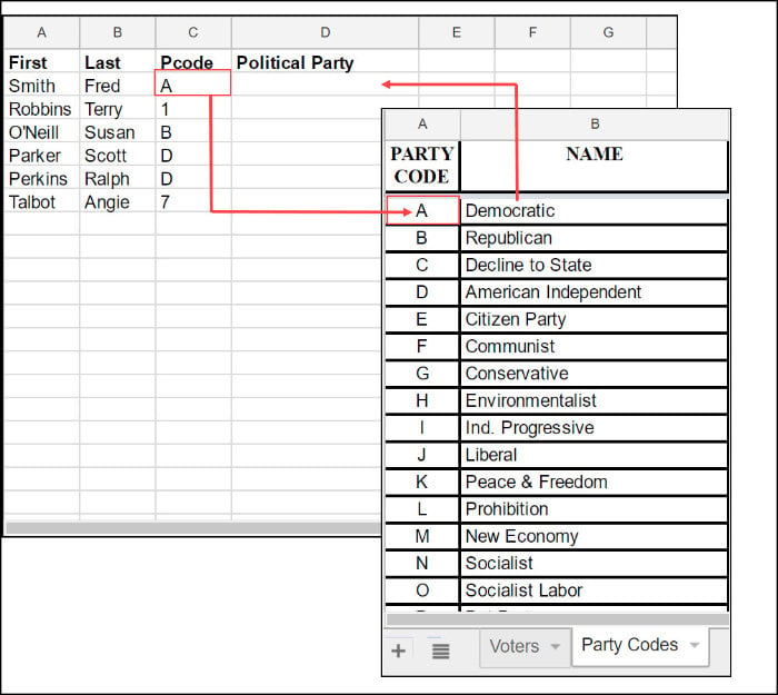
In the picture below, can you guess what a Pcode is?

It’s a code that represents the voter’s political party. You wouldn’t guess that unless you saw a related spreadsheet with additional information. Below you can see that the value in Pcode value above is the same as the value in PARTY CODE column.

What would make more sense is to add a column to the first Google worksheet that displays the political party name from the second worksheet. Using named ranges and the VLOOKUP function, we can improve our Google Sheet.

Part 1 – Map Our Spreadsheet Fields

When building a Google Sheets vlookup formula, it helps to define what you want and where the values are stored. You’ll see that column order impacts the results.

In my case, I want to:

1. Add a column to my Voters Google worksheet called Political Party
2. Look at a voter’s Pcode and find its corresponding NAME on the Party Codes worksheet
3. Copy that NAME to the voter’s Political Party column
4. Repeat the process for each voter.

Stating it another way, we’ll grab the voter’s “Pcode” and search column A for a matching value in the “PARTY CODE” column on the other worksheet. In this instance, the Pcode is our search key, and the Party Code column is our lookup column.

If we find an exact match, we’ll scan across in the “NAME” column and copy that value to the voter’s “Political Party” cell.

Before we begin, there are several important rules to know about the reference column you need to look up. In our case, this will be the PARTY CODE column on the Party Codes worksheet.

• The PARTY CODE column must be the left-most or first column.
• The PARTY CODE column values must be unique.
• The PARTY CODE column should be sorted. This also helps performance.

For example, I shouldn’t have the PARTY CODE column with multiple instances of the letter “A.” As you’ll see in the practice file, the values in this column are sorted starting with numbers and then letters.

Part 2 – Import the VLOOKUP Practice File

To make this tutorial easier, I’ve created a sample spreadsheet. You can right-click it and choose Save link as….

1. Open a new Google Sheet by typing sheet.new in your browser’s address bar.
2. From the File menu, select Import.
3. From the Import file dialog, click Upload.
4. Upload the sample tutorial file referenced above.
5. On the Import location dropdown menu select Replace spreadsheet.
6. Click the Import data button.

Part 3 – Create a Named Range in Google Sheets

If you’re not familiar with a named range, it’s a way of defining a cell range using meaningful names instead of absolute cell references. This becomes very handy when you reference ranges in formulas.

Instead of having a reference like 'Party Codes'!A2:B45 we can use a named range called PartyTable.

1. On the example spreadsheet, click the Party Codes tab.
2. Click cell A1.
3. Press Ctrl + A or command ⌘ + A to highlight the range.
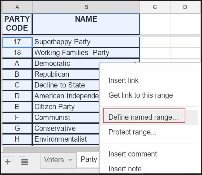
4. Right-click and select Define named range…. You may have to scroll a bit to see this option.

5. The Named ranges dialog will appear on the right. Change the name to PartyTable and click Done.

Part 4 – Build the VLOOKUP Formula

The VLOOKUP function has 4 arguments. The last item, Is-sorted, is optional but critical. This TRUE/FALSE value specifies our matching precision. By default, Google will use a TRUE value that matches a close value. That’s probably not a good idea when it comes to politics.

Argument	Meaning
Search_key	Which cell do we use Google Sheets VLOOKUP?
Range	Where should we look for the values? This is your lookup range.
Index	Which column number holds the value we need? This is our lookup column.
Is_sorted	Should we use “close match”? If this is set to FALSE, an exact match is returned. If TRUE, an approximate match is used.

1. On the Voter’s sheet, add your Political Party column in column D.
2. Click cell D2.
3. Start typing =vlookup. You may prefer to use the Google Sheets formula bar above the column headings. It has a more visible area for typing.

4. Type (.
5. Click cell C2. This is our Search_Criterion.
6. Type a , to separate our arguments.
7. Type PartyTable. This Named Range is our Array.
8. Type another ,.
9. Type 2. This is our Index. We’re telling Google to search for the values in the 2nd column on our Array.
10. Type another ,.
11. Type FALSE. This is our Sort_order. The FALSE means we want an exact match.
12. Type closing ).

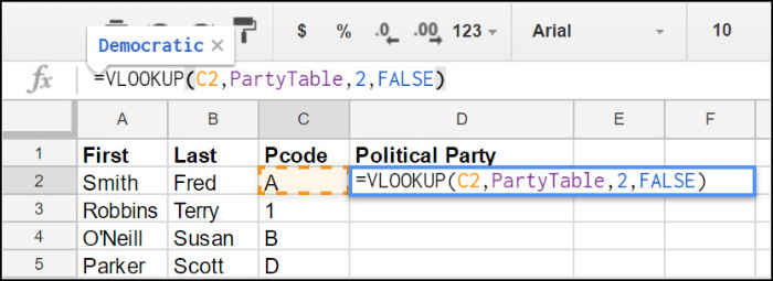
In the example above, Google Sheets shows the lookup value of “Democratic” in the formula bar. This indicates the formula found a lookup value.

13. Click Enter to commit the function.
14. Click and drag the sizing handle (blue square) on D2 down the column to copy the formula to the other cells.

Troubleshooting Google Sheets Formulas

Recently, a viewer contacted me saying the VLOOKUP formula didn’t work, and he shared a link to his Google Sheet with me. Sure enough, I couldn’t get the formula to work either. However, I could get it to work when I created the same Google Sheet on my end.

Interestingly he questioned whether his being in Italy made a difference. I said I didn’t think so because it would be a support issue for Google. They would want to be consistent. Long story short, he was right, and I was wrong.

If you click the File menu and go to File Settings, you’ll see a dialog similar to the one below.

It seems certain countries don’t like using commas in Google Sheets formulas. Instead, they need a semicolon. So, make sure your location is correct. If it is, try substituting a ; for ,. You may also need to add a space bar after the semicolon too. Google has a support article on this location issue.

Think of the VLOOKUP function as a detective for your data in Google Sheets, always searching for the right match. It’s an invaluable tool that bridges gaps between related data points. Master it, and you’ll turn your spreadsheets into well-connected, informative hubs.

If you find VLOOKUP formula in Google Sheets too restrictive there is another option – XLOOKUP. I haven’t done a tutorial yet, but take a look at my tutorial, How to Use XLOOKUP in Excel.

Hand-picked Tutorials

• Test Before Importing Google Contacts
• How to Remove Chrome Extensions
• How to View Your Chrome Browser History
• How to Make a Letterhead with Google Docs
• How to Bulk Delete Gmail Items