Are you looking to generate random numbers in Excel without the hassle? Whether it’s for data sampling, assignments, or selection tasks, I’ll show you 3 reliable methods to generate random numbers. Plus, discover an extra function that makes the process even easier for Microsoft 365 users.
Knowledge You’ll Gain:
- Understand the Key Principles of Random Number Generation in Excel
- Learn How to Confidently Use Excel’s RAND Function
- Become Proficient at Utilizing Excel’s RANDBETWEEN Function
- Prevent duplicate random numbers
- Learn about Microsoft 365 function -RANDARRAY
While other software programs have a random number generator, I chose Microsoft Excel because that was the source file format I received. If you want to get technical, I’m really dealing with pseudo-random number. For my purposes, I wasn’t worried about the differences.
Understanding RAND & RANDBETWEEN
Excel’s RAND function is a pretty simple and popular function on the surface. As you can see below, simply typing =RAND() in a cell produces tiny random decimal values which don’t appear to fit a normal distribution.
- 0.19934724
- 0.796184684
- 0.717061354
- 0.32105009
- 0.221891585
I prefer a random integer or whole numbers, so I chose another Excel Math & Trig function called RANDBETWEEN. You may need to install the Analysis Toolpak add-in.
One advantage of RANDBETWEEN is you specify a minimum value and a maximum value for your arguments. For example, =RANDBETWEEN(1,5000) would generate random whole numbers between 1 and 5000. This is important as you don’t want to duplicate values. It’s best to choose a top value much higher than you need. That way, the odds of getting the same random number are less.
I can add a spreadsheet column with either Excel function and create a random value for each row alongside the person’s name. That column can then be used to sort the list.

TextExpander: Worth It? Find Out.
Is TextExpander the right tool to boost your productivity? Get an independent assessment, weigh the pros and cons, and make an informed decision. Find out why I’m a fan.
Read the ReviewGenerate Random Numbers Step-by-Step
In the instructions below, I’ve started with a random list of US presidents and wish to randomly select 5 based on the smallest value of a random number I’ll create.
- Open your Excel spreadsheet.
- Add a column for Order in Column A.
- Add a Random number column in C.
- From the Formulas menu, select Calculation Options.

- Select Manual calculations.
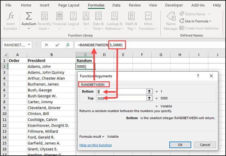
- In cell C1, type =RANDBETWEEN(1,5000). Alternatively, you may use the Insert Function button and fill out the Function Arguments dialog as below.
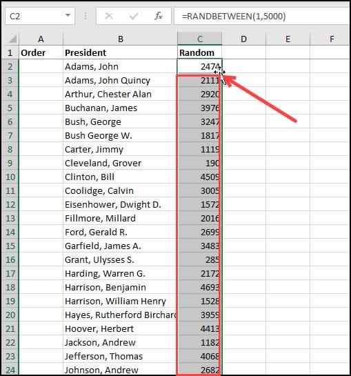
- Double-click the lower-right corner of C2. This will copy the Excel formula down the column.
- In cell A1, type 1.
- In cell A2, type 2. This is to establish the sequential number pattern.
- Double-click the lower-right corner of cell A2. This should fill in the original order range for your column.

- Click the Select All button. It’s the green triangle above the numbered rows.
- From the Data menu, select Sort. I opted to go from Smallest to Largest.
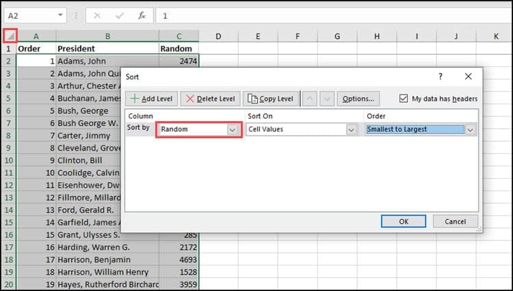
- Click OK.
- From here, I can select how many rows are needed, such as 5.
Introducing RANDARRAY (Microsoft 365)
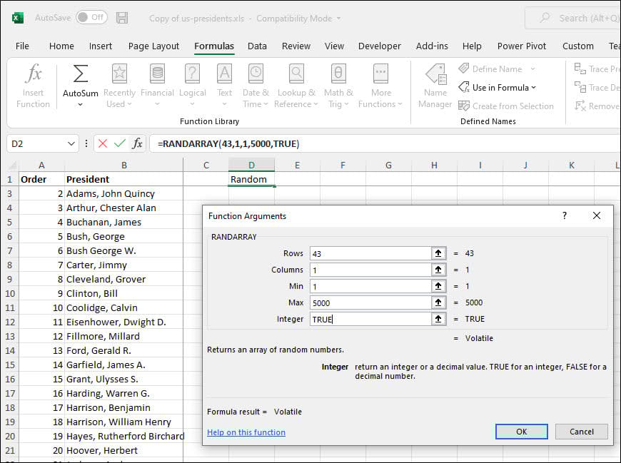
In 2020, Microsoft introduced another function for Microsoft 365 users called RANDARRAY. It is more versatile than RAND and RANDBETWEEN. For example, in addition to calculating random numbers, the function can also random names from an Excel named range.
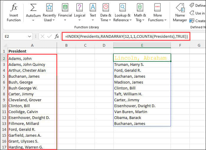
Or, if I preferred, I could select random numbers as before. The rows is the number of presidents. And by using TRUE in the Integer field, I will get whole numbers.
Tips & Troubleshooting for Random Numbers
The main point to remember about using either randomizer function is to turn off Excel’s automatic recalculation. Otherwise, having the random number in Excel update each time you open the worksheet is too easy. If that poses a problem, copy the Random column to a new one and use Paste Special Values. However, you’ll no longer have the underlying formula.
RANDBETWEEN poses another issue if you use small values. For example, I first used =RANDBETWEEN(1,50), figuring the range was larger than the number of presidents. However, I soon discovered it produced duplicate number values.
Now that you’ve learned Excel’s random number generation tools, you can confidently tackle any selection task that comes your way. Whether you choose the straightforward RAND function, the versatile RANDBETWEEN, or the powerful RANDARRAY (for Microsoft 365 users), you know how to generate reliable random numbers while avoiding common pitfalls like duplicate values.
Ready to explore more Excel techniques? Check out our related tutorials below.
