Are you looking to enhance your data analysis skills in Excel? Excel slicers could be the tool you need. This feature, one of my favorites, allows you to filter data in your Excel tables or pivot tables in a variety of ways. Think of it as an interactive dashboard at your fingertips. (Includes practice worksheet.)
What is an Excel Slicer?
This feature is similar to what you might encounter with an online movie guide. For example, your content provider might have buttons that filter for mystery, comedy, romance, or other genres. Slicers work similarly; users can easily choose multiple options to filter data on an Excel or pivot table.
Differences Between Slicers & AutoFilter
You might be thinking this feature sounds a lot like an Excel autofilter. There are similarities as both filter data. AutoFilter controls reside on the top of your columns. The slicers can reside in other locations and can be more descriptive. You can even have multiple button selectors.

These slicer buttons can make it easier to interact with your data table. It’s also more visual because you can see which filters are enabled. However, slicers can only be used on an Excel Table or PivotTable.
The Practice Workbook
For this Slicer tutorial, I’ll use a baseball database from Sean Laham containing 100+ years of stats. To make the table, you can download the Excel workbook with the three sheets:
Autofilter – worksheet using AutoFilter.
Practice – starting worksheet you can use for these instructions
Slicers – finished worksheet with 3 slicers
The underlying data is the same on all 3 sheets. The difference is in the presentation.
Start with an Excel Table
As mentioned, the slicer data objects can only be used with a table or an Excel Pivot table. For that reason, you won’t see the Slicer button enabled on either the Autofilter spreadsheet or the Practice spreadsheet.
- Download the Excel slicer tutorial worksheet.
- Click Enable editing at the top of Excel.
- Click the Practice tab at the bottom.
- Click the Insert tab from the ribbon.
- Click Table from the Tables group.
- The Create Table dialog opens. Keep the default entries and click OK.
Based on your table styles, you’ll see column filters at the top and rows with alternating color bands.
If you use your own spreadsheet file, it’s best to have single-row headers and no blank columns.
Add the Excel Slicer
Now that we have the table, we can start to add our slicers. You can have a slicer for each column. However, one benefit is that you can limit the number of slicers. Based on your data table, this might make the information easier to work with.
- Click table cell O2. From the Tools group, click Insert Slicer.
- A small Insert Slicers popup appears with a checkbox for each of your columns.

- Tick Team, Year, and League.
- Click OK.
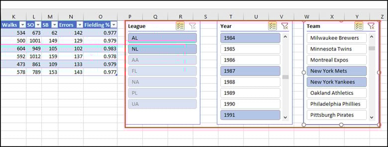
- Excel will create a small slicer for each item with their data cell entries.
- Position the Slicer Boxes someplace convenient such as a blank area to the right of the columns.
You will get a Report Connections error if you click a cell off the table area before clicking Insert Slicers. The toolbar is also context-aware, so if you don’t see Insert Slicer in the Tools group, click Insert and then Slicer from the Filters group.
Positioning the Slicers
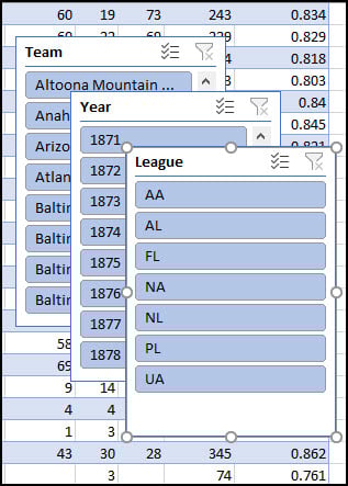
I prefer to lock my slicers’ positions so they are always at the top of the screen. In the top image, I had all the slicer boxes aligned at the top. Alternatively, I could drag the second slicer (Year) underneath League.
To disable the slicers from moving,
- Position and resize your slicers to the desired location.
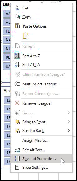
- Right-click on the Slicer title.
- Select Size and Properties… from the drop-down menu.
- In the Format Slicer box, toggle Position and Layout.
- Tick the checkbox for Disable resizing and moving.
- Repeat for your other slicers.
Understanding Slicer Elements
Each slicer has 5 areas.

[A] Slicer name. In this example – Team.
[B] Multi-selection icon. You can click to toggle On or Off. It’s currently On, as indicated by the yellow color.
[C] Filter reset icon to clear filter.
[D] Your current selections. These show in a different color.
[E] Scroll bar
You can also right-click a slicer to change its properties, such as formula name, header, caption, sorting, and empty cells. For example, you may prefer to have the Years slicer sorted in descending order. Additionally, you can filter out items with no data.
Making Multiple Selections
One useful feature is the ability to multi-select items. When you first start, your slicer will include all options. Sometimes, you end up with a different selection than what you expected.
Instead of just choosing one baseball team or year, you can opt to make several. For example, you might want to create a Region or Department slicer on one of your favorite spreadsheets.
To make multiple selections,
- Make your first selection.
- Click the Multi-select icon to the right of the Slicer name. The icon will turn yellow. I tend to have the best results when I turn on this feature. However, there are times when I’ve clicked multiple entries, and they’ve been enabled without using this toggle.
- Hold your Ctrl key down and click additional items.
Understanding Slicer Sorting
One of the best ways to understand how slicers interact with your data is to experiment. A connection remains between the table column filters and your slicer boxes. If you were to clear a slicer filter, you would see it impacts the other slicers and record count.
The easiest way to see this is to click the Filter reset icon on each slicer. You’ll then see every slicer item is enabled. Essentially, you’re seeing all the data.
Now, if you go to Column G – WSWin (Word Series winners) and filter for Y, the slicers on the right have changed. Instead of all the Leagues being enabled, only AA, AL, and NL are. The table shows 120 matching records. If you then select only the NL from the League slicer, the record count drops to 53. As you can see, you can use column filters and slicers together.
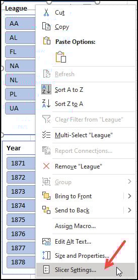
At this point, you may want to change the order of the Year slicer. Some people prefer ascending order and some descending order. You can right-click the Year title and select Slicer Settings from the drop-down menu. The Slicer Settings dialog box appears.
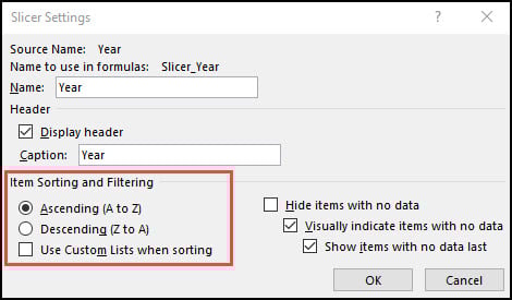
Since this collection spans over 100 years, you might change the Item Sorting and Filtering options. There are three options. Ascending, Descending, and Custom List.
A custom list is where you define the order. It doesn’t make sense in our tutorial unless you wanted a custom order for League based on the time period. Given that the list is 7 entries, it’s probably overkill.
As you can see, Excel slicers don’t change your cell data. Instead, they provide a convenient way to drill down to present a different perspective.