Do you feel like your Excel spreadsheet is a “hot mess” of data? Is it hard to find what you’re looking for? If so, the AutoFilter function can help. The Excel AutoFilter allows you to filter through your spreadsheets and display only the information that meets certain criteria. In the tutorial below, I’ll show how to turn on automatic filters in Excel.
Why Use Filters
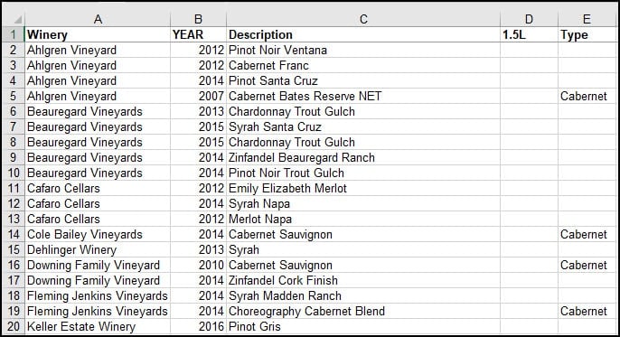
For example, let’s say your boss owns a wine shop and just got a wine shipment. Your task is to restock the shelves. However, you also know that someone from marketing will call in the next couple of days to ask about these wines.
Taking a proactive approach, you add two columns to the Excel spreadsheet. The first task is to stock the shelves. The wine description field hints at varietal and bottle size. These values are important for stocking, especially since the 1.5-liter bottles don’t fit the standard shelves. So you add two columns to the Excel sheet for “1.5L” size bottles and “Type.”
Although we’ve added the new columns, we can be more productive by adding some column filters. The column filters will allow us to drill down to find entries and answer questions. No more scrolling through countless spreadsheet rows.
TextExpander: Worth It? Find Out.
Is TextExpander the right tool to boost your productivity? Get an independent assessment, weigh the pros and cons, and make an informed decision. Find out why I’m a fan.
Read the ReviewWhat is AutoFilter?
AutoFilter is an easy way to turn the values in an Excel column into filters based on the column’s cells or content. For example, by adding AutoFilter to the worksheet above, I could filter the “Winery” column to only display rows from Beauregard Vineyards. All the other wineries stay on the Excel worksheet but don’t display. Unlike Excel Slicers, which work on Excel Tables or Pivot Tables, Autofilter works everywhere.
To turn on AutoFilter,
- Click any cell within your range.
- From the Data tab, click Filter. It’s in the Sort & Filter panel.

Once you’ve enabled this feature, your columns display with a drop-down arrow to the right. If you click the arrow control, you’ll see all the values for that particular column. To turn off AutoFilter, click Filter from the Sort & Filter panel again.
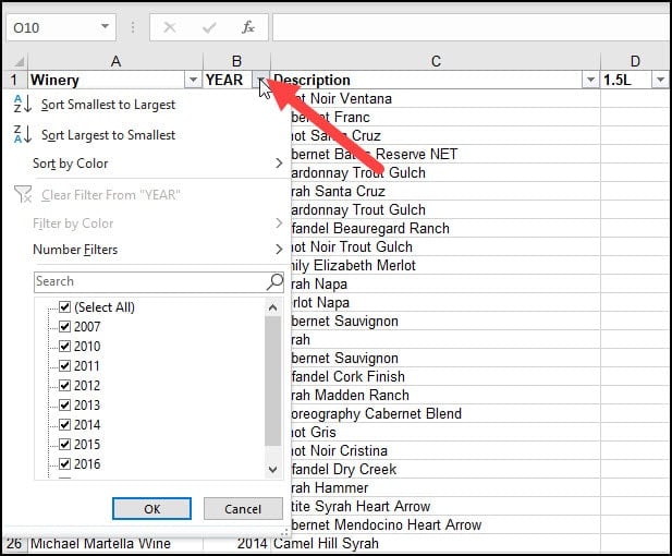
In the example above, I can see all the values that show in the YEAR column. However, various years are omitted since the spreadsheet doesn’t represent the values. In other words, 2008 doesn’t show because no cells are containing that data.
What’s appealing about this filter feature is that the displayed list is dynamic. For example, if I shift to the 1.5L column, you’ll see my options vary and include an item for blank cells.

What’s equally useful is these filters also adjust based on other autofilters. So, for example, if I filter the “Winery” column for “Ridge Vineyards” as shown below, my autofilter list for “YEAR” only displays Ridge values.

Excel Custom AutoFilters
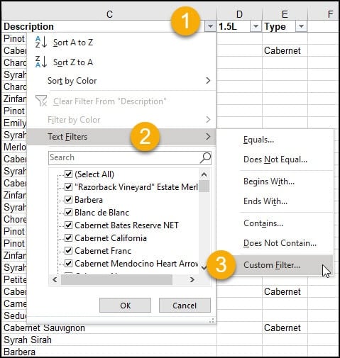
As handy as these filters are, there are times when you need to filter based on specific criteria within a cell. For example, we can use a custom filter to filter by wine type. This works because the distributor gives hints in the “Description” line.
To set a simple custom autofilter,
- Enable autofilter for your spreadsheet using the steps in the section above.
- Next, click the down control arrow in the column you wish to filter. [1]
- From the drop-down list, select Text Filters [2]. The wording may change based on the column contents.
- From the side menu, select Custom Filter… [3]
- The Custom AutoFilter dialog should appear.
- Click the drop-down arrow in the first list box and select your criteria.
- In the list box to the right, either type a value or select one from the list.
- Click OK.
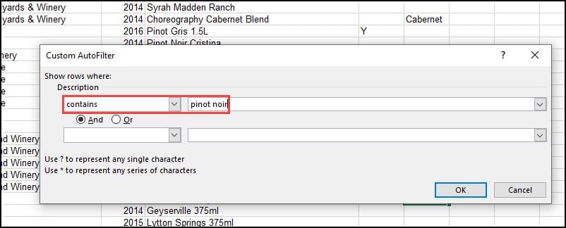
In the example below, I’ve elected to filter for rows containing “pinot noir” anywhere in the description. Once my filtered rows appear, I’ll add “Pinot Noir” in the Type column.
Excel is versatile in the filter settings. You’re not limited to just items containing a specific value. The choices change based on the column’s data type. You could also use:
- equals
- does not equal
- is greater than
- is greater than or equal to
- is less than
- is less than or equal to
- begins with
- does not begin with
- ends with
- does not end with
- contains
- does not contain
Refining Excel Filters with Radio Buttons
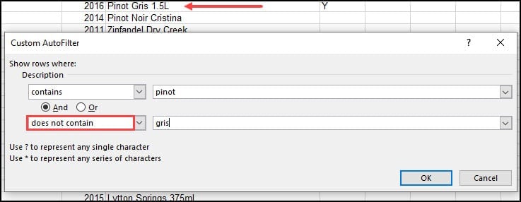
Sometimes you need a more complicated filter. For example, I may want to select a row if two conditions are met. I might also be interested in selecting a cell if one or another condition is met. Excel allows you to refine your filter using the AND and OR radio buttons.
Using our wine store example, I might want to filter wines with Pinot in the description but not Pinot Gris. The procedure is similar to the above, but I added another condition and used the “And” radio button. My second condition also uses the “does not contain” option.
Once I’ve filtered for a specific wine term(s), I can quickly enter the value in the “Type” column for the resulting set. I can repeat this process for each wine type, such as Zinfandel, Syrah, Chardonnay, and so on. You may meet some examples that don’t fit your filters. For example, in my spreadsheet, some descriptions, such as Monte Bello, don’t show the type of wine.
Essentially, Excel’s autofilters allow you to slice and dice your rows. The only limitation is if you have more than 1000 unique items in a list. It won’t help you empty the wine boxes but can help you decide where items should go. So if you find some Monte Bello, save it for a special occasion. One when you’re far away from a computer.
If you ever need to see your Excel autofilter settings, we did a separate tutorial on the subject.