Microsoft Excel is the go-to spreadsheet for many. However, some data entry methods lead to errors. One example is when you want to restrict the entries on an Excel drop-down list based on a previous condition. This tutorial will show how to create a dependent Excel drop-down list to avoid errors. (Includes practice worksheet)
What is a Dependent Drop List?
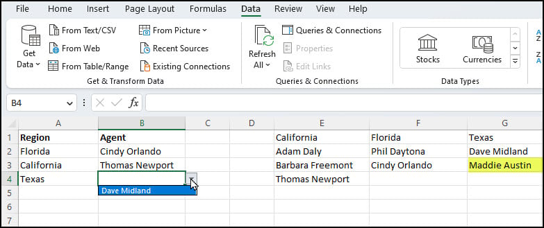
In the screen example below, there are two lists. Column A is the Region, and Column B is the Agent. The 2nd list or Agent list is dependent on the Region. So, for example, if you select Florida on A4, you will only see Florida agents when you click B4. You won’t see agents from other states.

Benefits of Excel Dependent Lists
There are many scenarios where these lists could be helpful. This conditional dropdown list approach has several benefits.
- The list items are restricted to valid entries.
- Finding the correct entry is faster because you’re not seeing all the agents. So, you might think of this as a conditional filter for the second drop-down list.
- You’re not typing so the data entry is faster.
- Google Sheets have similar functionality if you ever switch programs.
I also think that using this type of conditional logic or dependency makes you plan your spreadsheet structure. Instead of entering everything free-form, you should take time and see if you have relationships. For example, while this tutorial only uses two lists, you could add more drop-down lists.
These lists differ from an Excel Custom List, which has no dependencies.
Setting Up the Worksheet
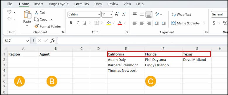
First, we’ll build a worksheet with two lists where the user can select a region (A). Then, the agent data (B), the dependent list, will be pulled from an Excel table (C) based on our selection.

We’ll use some features and simple formulas we’ve discussed before to build these lists. I also used Microsoft 365, but earlier Microsoft Excel versions will work.
- Named Ranges
- Data Validation
- Excel tables
- INDIRECT Function
To start, enter the same data that shows in Figure 1 above. You don’t need to add any formatting.
Add Functionality with an Excel Table
Before we build our dependencies, I want to convert the state agent list (C) into a table. Excel Tables have many benefits, but in this case, they will allow us to expand the source list dynamically.
For example, if I add Maddie Austin in G3 as a Texas agent, her name will not appear in the dependent dropdown. I would have to make adjustments.

To Create the Excel Table,
- Highlight cells E1:G4. This is our header row.
- Press Ctrl + T.
- In the Create Table dialog box, tick the checkbox for My table has headers.

- Click OK.
Changing Table Name (Optional)
I prefer to name my tables. It makes it easier when I’m looking in the Name Manager. I also turned off Banded Rows. However, you want to keep the Header Row.
- Click any table cell.
- Click the Table Design tab.
- In the far left, type your entry in the Table Name textbox such as “Agents”.

Defining the Region (States)
A key component of using dependent lists is to create a named range. When we do our data validation, we will be referencing it. In our example, we want a named range that equates to the states.
- Click Formulas on the ribbon.
- Highlight cells E1:G1. This is your Header Row representing the current states.
- In the Defined Names group, click Define Name.
- In the New Name dialog box, enter “Region” for the Name.

- Click OK.
Building the Region Drop Down List
Next, we want to build a drop-down list for the user that allows them to select a pre-defined state. We only want the user to see California, Florida, and Texas. They shouldn’t be able to enter anything else in Column A. This is done by using data validation.
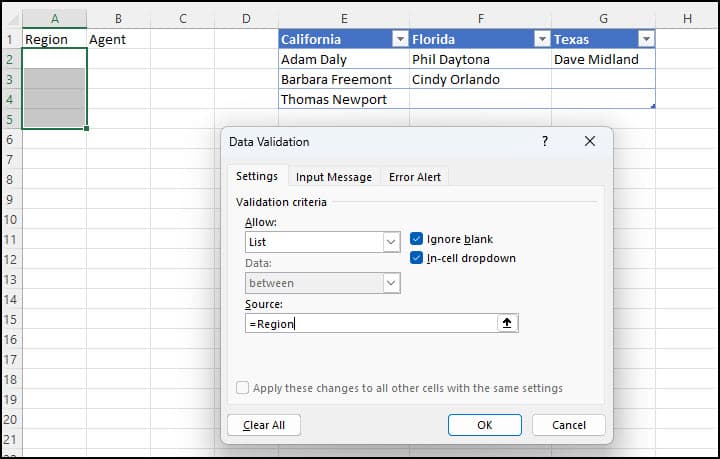
- Highlight cells A2 through A5.
- Click the Data tab from the ribbon.
- In the Data Tools group, click Data Validation.
- From the Settings tab in the Data Validation dialog box, change the Allow value from Any value to List.
- Click in the Source: text box.
- Press F3. The Paste Name dialog box appears.
- Click Region.

- Click OK.
By using F3, you limit spelling mistakes.
Testing the Region List
Even though I used F3 to ensure I didn’t misspell the name, this is a good time to test.
- Click cell A2.
- You should see a drop-down control ▼ to the right side.
- Click the drop-down list control.
- Verify the list shows: California, Florida and Texas.
Creating State Named Ranges
Although we defined a region list, we must define named ranges for the states to build the dependency. We’ll start with California.
- Highlight cells E1:E4.
- Click the Formulas tab.
- In the Defined Names group, click Create from Selection.
- In the Create Names from Selection dialog, tick Top row.
- Click OK.
- Repeat the above steps for Florida (F1:F3) and Texas (G1:G2).
If you press Ctrl + F3, you can see all your Named Ranges and Table Names.

Using an INDIRECT Formula to Validate
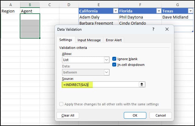
Now, we want the create the dependent drop-down list. While the states are showing in the Region column, nothing is happening for Agent. No California agents show. Again, we’ll use a data validation formula using the INDIRECT function and a cell reference.
- Highlight cells B2 to B5.
- Click the Data tab.
- Click Data Validation.
- On the Settings tab change the Allow: field from Any value to List.
- In the Source: textbox type =INDIRECT($A2)

- Click OK.
If you get a data source evaluation error that reads, “The Source currently evaluates to an error. Do you want to continue?” It’s most likely caused by an empty cell in A2. Click Yes.

Testing the Dependent List
- Make sure cell A2 is California.
- Click cell B2.
- Click the drop-down control to the right.
- Verify you see California agents.

You can use cells A3:A4 to test Florida and Texas.
Adding More States and Agents
As I mentioned, this was a simple scenario. However, you may have a situation where you need to add more agents for a state or even new states.
Since we used an Excel table for the state agents, you could add agents by typing their names under the respective state. So, for example, I could add “Sue Sunnyvale” in cell C5, and she would show in the Agent dropdown list for California.
One difference is when I add a state. For example, if I type Virginia in cell H1, it will appear on the Region list. But if I add new Virginia agents, I must go back and define a named range for Virginia as we did with the other states.
One caveat is you can’t have a defined name with a space. So, while I can add “West Virginia,” and it will show in the Region drop-down list, nothing will show on the Agents dependent list. This is a limitation of these lists. The easiest workaround is to use an underscore.
Hopefully, you see the value of these conditional drop-down lists in Excel. Although they take a little time to create, the dependent drop-down list can save you from making errors and speed up your data entry.
